Chapter 4 Post-surgery

4.1 BRE

plot.info <- read.xlsx("data/TableS6.xlsx", startRow = 3)
colnames(plot.info)[1:3] <- c("Sample","Disease","GroupHormone")
colnames(plot.info) <- str_replace_all(colnames(plot.info), regex(".\\(.+"), "")
colnames(plot.info) <- str_replace_all(colnames(plot.info), regex("/"), "_")

sub.1 <- plot.info[, c(1:3, 19, 4:18)]
sub.1$Group <- "Before"
sub.2 <- plot.info[, c(1:3, 19, 20:34)]
sub.2$Group <- "After"

plot.data <- rbind(sub.1, sub.2)
plot.data$Group <- factor(plot.data$Group, levels = c("Before","After") )

plot.data$Time <- factor(as.character(plot.data$Time), levels = c("day2","day3","day4","day5","day6","day30"))
table(plot.data$Time)

## 
##  day2  day3  day4  day5  day6 day30 
##    44    82    62    34   126    52

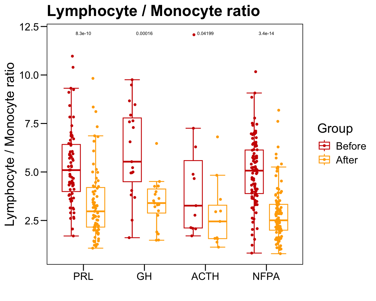
p <- ggboxplot(plot.data, 
               x = "GroupHormone", y = "Lymphocyte._.Monocyte.ratio",
               color = "Group", fill = "white",
               palette = c("#CE0000","#ffaa00"),
               order = names(color.hormone),
               width = 0.6, bxp.errorbar = TRUE, bxp.errorbar.width = 0.5,
               add = "jitter", add.param = list(color = "Group", size = 1, width = 0.5),
               xlab = "", ylab = paste0( "Lymphocyte / Monocyte ratio" ),
               main = paste0( "Lymphocyte / Monocyte ratio" ),
              legend = "bottom" )
p <- p + stat_compare_means(aes(group = Group, label = paste0(..p.format..)), method = "wilcox.test", paired = T, size = 2 )
p <- p + theme_base() + theme(plot.background = element_blank())
p

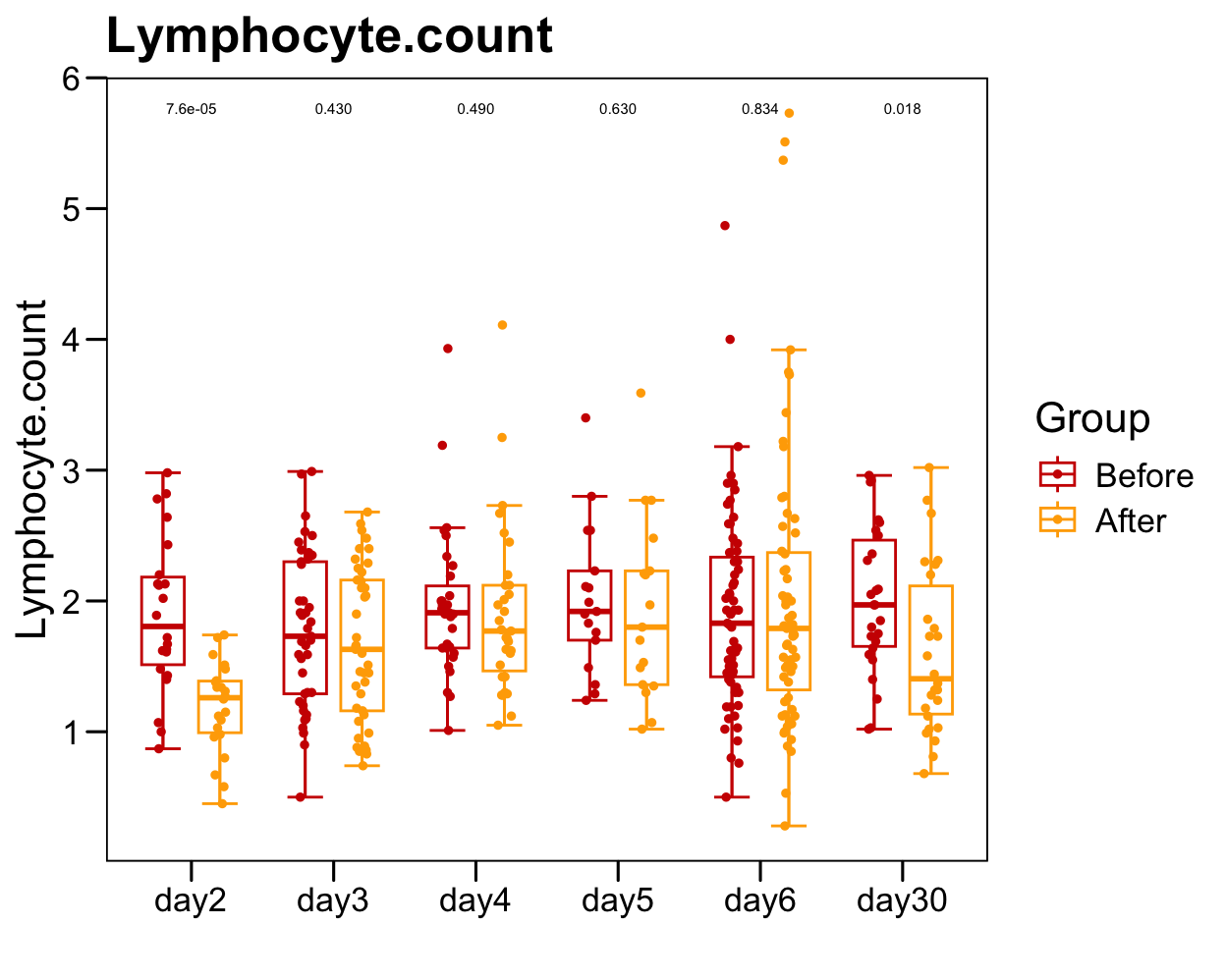
p <- ggboxplot(plot.data, 
               x = "Time", y = "Lymphocyte.count",
               color = "Group", fill = "white",
               palette = c("#CE0000","#ffaa00"),
               width = 0.6, bxp.errorbar = TRUE, bxp.errorbar.width = 0.5,
               add = "jitter", add.param = list(color = "Group", size = 1, width = 0.5),
               xlab = "", ylab = paste0( "Lymphocyte.count" ),
               main = paste0( "Lymphocyte.count" ),
               legend = "bottom" )
p <- p + stat_compare_means(aes(group = Group, label = paste0(..p.format..)), method = "wilcox.test", size = 2 )
p <- p + theme_base() + theme(plot.background = element_blank())
p

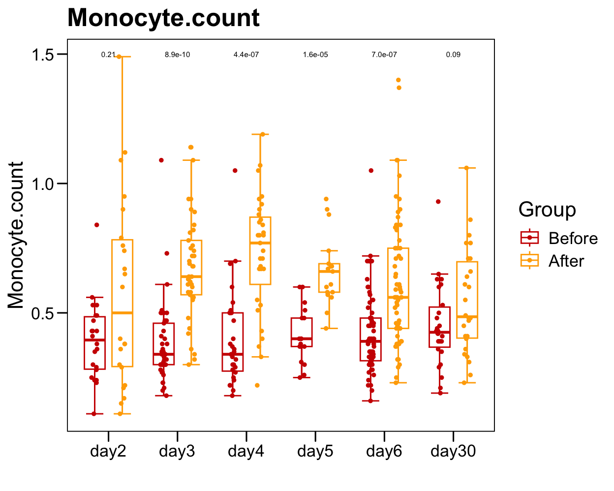
p <- ggboxplot(plot.data, 
               x = "Time", y = "Monocyte.count",
               color = "Group", fill = "white",
               palette = c("#CE0000","#ffaa00"),
               width = 0.6, bxp.errorbar = TRUE, bxp.errorbar.width = 0.5,
               add = "jitter", add.param = list(color = "Group", size = 1, width = 0.5),
               xlab = "", ylab = paste0( "Monocyte.count" ),
               main = paste0( "Monocyte.count" ),
               legend = "bottom" )
p <- p + stat_compare_means(aes(group = Group, label = paste0(..p.format..)), method = "wilcox.test", size = 2 )
p <- p + theme_base() + theme(plot.background = element_blank())
p

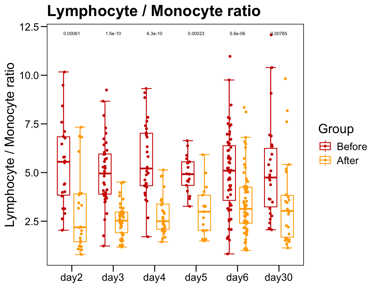
p <- ggboxplot(plot.data, 
               x = "Time", y = "Lymphocyte._.Monocyte.ratio",
               color = "Group", fill = "white",
               palette = c("#CE0000","#ffaa00"),
               width = 0.6, bxp.errorbar = TRUE, bxp.errorbar.width = 0.5,
               add = "jitter", add.param = list(color = "Group", size = 1, width = 0.5),
               xlab = "", ylab = paste0( "Lymphocyte / Monocyte ratio" ),
               main = paste0( "Lymphocyte / Monocyte ratio" ),
               legend = "bottom" )
p <- p + stat_compare_means(aes(group = Group, label = paste0(..p.format..)), method = "wilcox.test", size = 2 )
p <- p + theme_base() + theme(plot.background = element_blank())
p

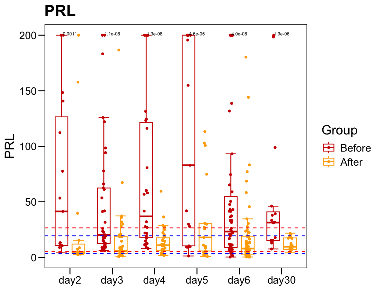
sub <- plot.data[which(!is.na(plot.data[, "PRL" ])), ]
sub.1 <- table(sub$Sample)
sub.1 <- sub.1[sub.1 > 1]
plot.data.sub <- plot.data[plot.data$Sample %in% names(sub.1), ]
table(plot.data.sub$Time)/2

## 
##  day2  day3  day4  day5  day6 day30 
##    15    37    30    17    55    20

p <- ggboxplot(plot.data.sub, 
               x = "Time", y = "PRL",
               color = "Group", fill = "white",
               palette = c("#CE0000","#ffaa00"),
               #order = c("FirstVisit", "LastVisit"),
               width = 0.6, bxp.errorbar = TRUE, bxp.errorbar.width = 0.5,
               add = "jitter", add.param = list(color = "Group", size = 1, width = 0.5),
               xlab = "", ylab = paste0( "PRL" ),
               main = paste0( "PRL" ),
               legend = "bottom" )
p <- p + stat_compare_means(aes(group = Group, label = paste0(..p.format..)), method = "wilcox.test", paired = T, size = 2 )
p <- p + theme_base() + theme(plot.background = element_blank())
p <- p + geom_hline(yintercept = normal.cutoff.male$PRL, linetype="dashed", color = "blue")
p <- p + geom_hline(yintercept = normal.cutoff.female$PRL, linetype="dashed", color = "red")
p

sub <- plot.data[which(!is.na(plot.data[, "GH" ])), ]
sub.1 <- table(sub$Sample)
sub.1 <- sub.1[sub.1 > 1]
plot.data.sub <- plot.data[plot.data$Sample %in% names(sub.1), ]
table(plot.data.sub$Time)/2

## 
##  day2  day3  day4  day5  day6 day30 
##    15    37    30    17    55    20

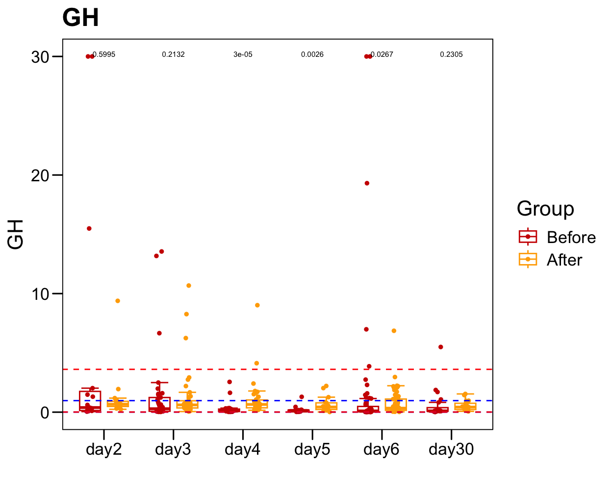
p <- ggboxplot(plot.data.sub, 
               x = "Time", y = "GH",
               color = "Group", fill = "white",
               palette = c("#CE0000","#ffaa00"),
               #order = c("FirstVisit", "LastVisit"),
               width = 0.6, bxp.errorbar = TRUE, bxp.errorbar.width = 0.5,
               add = "jitter", add.param = list(color = "Group", size = 1, width = 0.5),
               xlab = "", ylab = paste0( "GH" ),
               main = paste0( "GH" ),
               legend = "bottom" )
p <- p + stat_compare_means(aes(group = Group, label = paste0(..p.format..)), method = "wilcox.test", paired = T, size = 2 )
p <- p + theme_base() + theme(plot.background = element_blank())
p <- p + geom_hline(yintercept = normal.cutoff.male$GH, linetype="dashed", color = "blue")
p <- p + geom_hline(yintercept = normal.cutoff.female$GH, linetype="dashed", color = "red")
p

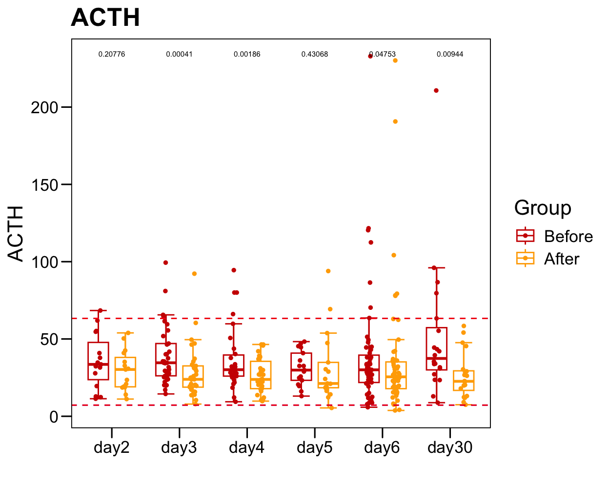
sub <- plot.data[which(!is.na(plot.data[, "ACTH" ])), ]
sub.1 <- table(sub$Sample)
sub.1 <- sub.1[sub.1 > 1]
plot.data.sub <- plot.data[plot.data$Sample %in% names(sub.1), ]
table(plot.data.sub$Time)/2

## 
##  day2  day3  day4  day5  day6 day30 
##    15    37    30    17    55    20

p <- ggboxplot(plot.data.sub, 
               x = "Time", y = "ACTH",
               color = "Group", fill = "white",
               palette = c("#CE0000","#ffaa00"),
               #order = c("FirstVisit", "LastVisit"),
               width = 0.6, bxp.errorbar = TRUE, bxp.errorbar.width = 0.5,
               add = "jitter", add.param = list(color = "Group", size = 1, width = 0.5),
               xlab = "", ylab = paste0( "ACTH" ),
               main = paste0( "ACTH" ),
               legend = "bottom" )
p <- p + stat_compare_means(aes(group = Group, label = paste0(..p.format..)), method = "wilcox.test", paired = T, size = 2 )
p <- p + theme_base() + theme(plot.background = element_blank())
p <- p + geom_hline(yintercept = normal.cutoff.male$ACTH, linetype="dashed", color = "blue")
p <- p + geom_hline(yintercept = normal.cutoff.female$ACTH, linetype="dashed", color = "red")
p

4.2 PitNET tissue

4.3 scRNA-seq

hypo <- readRDS("data/20250925_PitNETs_scRNA_tissue_s63.rds")

p <- DimPlot(hypo, reduction = "umap", pt.size = pt.size, raster = set.raster, label = T, label.size = 4,
             group.by = "Sample", cols = color.lib, shuffle = T) + theme_few()
ggsave(paste0(out.path, "/5.UMAP.sample.png"), p, width = 11, height = 7, dpi = 300)

p <- DimPlot(hypo, reduction = "umap", pt.size = pt.size, raster = set.raster, label = T, label.size = 3,
             group.by = "CellType", cols = color.tumor) + theme_few()
ggsave(paste0(out.path, "/5.UMAP.CellType.png"), p, width = 10, height = 7, dpi = 300)

p <- DimPlot(hypo, reduction = "umap", pt.size = pt.size, raster = set.raster, label = T, label.size = 4,
             group.by = "Branch", cols = color.branch) + theme_few()
ggsave(paste0(out.path, "/5.UMAP.Branch.png"), p, width = 8.5, height = 7, dpi = 300)

4.4 inferCNV

infercnv_obj <- infercnv::CreateInfercnvObject(raw_counts_matrix=count.cnv, 
                                               gene_order_file=genes.cnv,
                                               annotations_file=annot.cnv,
                                               ref_group_names = rev(c("Normal_cell")) )

infercnv_obj_default = infercnv::run(
  infercnv_obj,
  cutoff=0.1, # cutoff=1 works well for Smart-seq2, and cutoff=0.1 works well for 10x Genomics
  out_dir=out.path.cnv,
  cluster_by_groups=TRUE, 
  plot_steps=FALSE,
  denoise=TRUE,
  HMM=FALSE,
  no_prelim_plot=FALSE,
  png_res=300,
  output_format = "pdf"
)
saveRDS(infercnv_obj, file = paste0(out.path.cnv, "/infercnv.CNV.obj.rds"))