Chapter 3 Target Evaluation
3.1 Load packages
library(openxlsx)
library(dplyr)
library(DT)
library(nlme)
library(DESeq2)
library(SummarizedExperiment)
library(openxlsx)
library(dendextend)
library(matrixStats)
library(data.table)
library(ggpubr)
library(limma)
library(DESeq2)
library(pheatmap)
library(gplots)
library(survminer)
library(survival)
library(enrichR)
library(stringr)
library(ggthemes)
library(fmsb)


# color theme
tp53.mutant <- c("WT","L130V","L130F","L130R","P142L","V143M","A161T","M237V","G245D","F270I","F270V","V272A","V272M","R248Q","R273H","null")
tp53.mutant.color <- c("red",rep("#494949","14"),"#E3E3E3")
names(tp53.mutant.color) <- tp53.mutant

anno.color <- list(
  Mutant = tp53.mutant.color)
3.2 Merge profiling
We provided the merged profiling, which could be downloaded via https://github.com/NRCTM-bioinfo/p53_compounds.
tp53.targets <- read.xlsx("01.Profiling/p53_targets.xlsx")
rownames(tp53.targets) <- tp53.targets$Gene

tp53.target.g32 <- tp53.targets$Gene[which(tp53.targets$LiteratureNum >= 10)]
tp53.target.g116 <- tp53.targets$Gene

merge.meta.data <- read.xlsx("01.Profiling/p53_meta.xlsx", sheet = 1)

merge.compare.data <- read.xlsx("01.Profiling/Table1.xlsx", sheet = 1, startRow = 2)
merge.compare.data$Sample <- merge.compare.data$`Sample.name.(after.treatment)`
merge.compare.data$Control <- merge.compare.data$`Sample.name.(untreated.samples)`
merge.compare.data$Group <- str_replace(merge.compare.data$Sample, regex("_rep.$"), "")
rownames(merge.compare.data) <- merge.compare.data$`Sample.name.(after.treatment)`

merge.mat <- read.xlsx("01.Profiling/Table2.xlsx", sheet = 1, startRow = 3, rowNames = T)
3.3 Normalization
# Median normalization
merge.nor.mat <- merge.mat
sub.1 <- aggregate(colMedians(as.matrix(merge.nor.mat)),
                   list(Cell = merge.meta.data$Dataset), min)
for (i in 1:ncol(merge.nor.mat)) {
  merge.nor.mat[, i] <- merge.nor.mat[, i] - sub.1$x[which(sub.1$Cell == merge.meta.data$Dataset[i])]
}


# Generation of fold change (Log2-transformed for FPKM) of cell line samples after treatment compared to before treatment
compare.mat <- NULL
for (i in 1:nrow(merge.compare.data)) {
  if (length(grep("; ", merge.compare.data$Control[i])) > 0) {
    sub.1 <- unlist(str_split(merge.compare.data$Control[i], "; "))
    sub <- merge.nor.mat[, merge.compare.data$Sample[i]] - rowMeans(merge.nor.mat[, sub.1])
  } else {
    sub <- merge.nor.mat[, merge.compare.data$Sample[i]] - merge.nor.mat[, merge.compare.data$Control[i]]
  }
  compare.mat <- cbind(compare.mat, sub)
}
colnames(compare.mat) <- merge.compare.data$Sample

head(compare.mat, 3)
## U937_WT U937_L130V_ATO U937_L130F_ATO U937_L130R_ATO U937_P142L_ATO U937_V143M_ATO U937_M237V_ATO
## CDKN1A 3.1916457 3.080478 1.957199 2.0917992 0.7774611 2.1667723 1.9077609
## RRM2B 0.8391627 1.001993 1.187001 0.6459767 0.4785670 0.8683713 0.5825729
## MDM2 2.7245150 2.028156 1.302068 1.1567997 0.8098108 1.5695778 1.3455218
## U937_F270I_ATO U937_F270V_ATO U937_V272A_ATO U937_V272M_ATO U937_V272M_PAT
## CDKN1A 3.947027 2.909291 2.035912 3.675682 3.269377
## RRM2B 1.860397 1.479516 0.708025 1.567485 1.557309
## MDM2 2.642251 2.444877 1.671464 3.256886 2.245890
## Kasumi-1_R248Q_Kevetrin_6h_rep1 Kasumi-1_R248Q_Kevetrin_6h_rep2 Kasumi-1_R248Q_Kevetrin_6h_rep3
## CDKN1A -0.00507247 -0.03563892 0.17165276
## RRM2B 0.66265896 0.57210179 0.51180155
## MDM2 0.04900353 -0.04690794 -0.01286232
## SKM1_R248Q_APR-246_rep1 SKM1_R248Q_APR-246_rep2 SKM1_R248Q_APR-246_rep3 staET7.1_R273H_APR-246_rep1
## CDKN1A -0.07281667 0.02994333 -0.26504667 0.4066695
## RRM2B 0.13078333 0.05577333 -0.27296667 0.6471832
## MDM2 0.18355667 -0.07633333 -0.09720333 0.2011240
## staET7.1_R273H_APR-246_rep2 staET7.2_R273H_APR-246_rep1 staET7.3_R273H_APR-246_rep1
## CDKN1A -0.31610198 -0.1298085 -0.41130580
## RRM2B 0.12121419 0.3475557 0.07482002
## MDM2 -0.04862277 0.1818754 0.07292721
## staET7.3_R273H_APR-246_rep2 staET7.2_R273H_APR-246_rep2 Saos-2_R273H_APR-246_6h_rep1
## CDKN1A -0.091652792 1.1191052 -0.02540054
## RRM2B 0.356190359 0.5005976 1.05526980
## MDM2 0.001335775 0.2663554 -0.08762767
## Saos-2_R273H_APR-246_6h_rep2 Saos-2_R273H_APR-246_6h_rep3 Saos-2_R273H_APR-246_12h_rep1
## CDKN1A -0.1177016 -0.534773959 -0.62120069
## RRM2B 1.1814193 0.431825568 1.03123586
## MDM2 0.3947754 -0.008325736 0.06401986
## Saos-2_R273H_APR-246_12h_rep2 Saos-2_R273H_APR-246_12h_rep3 Kasumi-1_R248Q_Kevetrin_48h_rep1
## CDKN1A -0.10077979 -0.3485730 0.3656561
## RRM2B 0.75826079 0.6167059 1.0807021
## MDM2 0.02695217 0.0326328 -0.4937894
## Kasumi-1_R248Q_Kevetrin_48h_rep2 Kasumi-1_R248Q_Kevetrin_48h_rep3 PCI13_G245D_COTI-2_rep1
## CDKN1A 0.6150592 0.5977127 0.7164330
## RRM2B 1.0029696 1.2170216 0.1130768
## MDM2 -0.5052966 -0.2238308 0.2377859
## PCI13_G245D_COTI-2_rep2 PCI13_G245D_COTI-2_rep3 U266_A161T_PRIMA-1_rep1 U266_A161T_PRIMA-1_rep2
## CDKN1A 0.6274429 0.647518846 0.1974164 0.4389011
## RRM2B -0.0679887 -0.006853216 -0.2733003 -0.3027616
## MDM2 0.2552303 0.341083919 -0.2199022 -0.2003108
## U937_R273H_ATO U937_R273H_PAT PCI13_G245D_CDDP_rep1 PCI13_G245D_CDDP_rep2 PCI13_G245D_CDDP_rep3
## CDKN1A 0.3927590 0.1909721 -0.21575276 -0.29477320 -0.3104395
## RRM2B 0.2643679 -0.1862437 -0.28507761 -0.56260138 -0.4041368
## MDM2 -0.5397466 -0.4929459 0.06734607 0.07106408 0.1046652
## 8266R5_null_PRIMA-1_rep1 8266R5_null_PRIMA-1_rep2 Saos-2_null_APR-246_6h_rep1 Saos-2_null_APR-246_6h_rep2
## CDKN1A -0.1462286 -0.1858493 1.0204064 -0.2922208
## RRM2B -0.2320481 0.2372455 0.2411493 0.4065886
## MDM2 0.2465478 0.3169312 -0.6160103 -0.6468282
## Saos-2_null_APR-246_6h_rep3 Saos-2_null_APR-246_12h_rep1 Saos-2_null_APR-246_12h_rep2
## CDKN1A 0.16556354 -0.252144504 -0.2329088
## RRM2B -0.31879809 0.490890719 -0.4246623
## MDM2 -0.05262877 0.001146008 -0.11603993.4 32 confident p53 targets
The heatmap plot was used for visualization of the log2-transformed fold change of 32 confident p53 targets.
my.breaks <- c(seq(-1.5, -0.01, by = 0.001), seq(0.01, 1.5, by = 0.001) )
my.colors <- c(colorRampPalette(colors = c("#00599F","#00599F","#287dba","#62aee5","#a8dcff","white"))(length(my.breaks)/2),
               colorRampPalette(colors = c("white","#ffca79","#ef6e51","#db1b18","#b50600","#b50600"))(length(my.breaks)/2))

plot.mat <- compare.mat[tp53.target.g32, ]
anno.data <- data.frame(row.names = merge.compare.data$Sample,
                        Mutant = merge.compare.data$p53.status)

# Visualization of the 32 confident p53 targets
p <- pheatmap(plot.mat, scale = "none",
              color = my.colors, breaks = my.breaks,
              cluster_row = F, cluster_col = F, border_color = NA,
              annotation_col = anno.data,
              annotation_colors = anno.color,
              clustering_method = "ward.D2",
              clustering_distance_rows = "manhattan",
              clustering_distance_cols = "manhattan",
              fontsize_col = 6,
              fontsize_row = 6)
p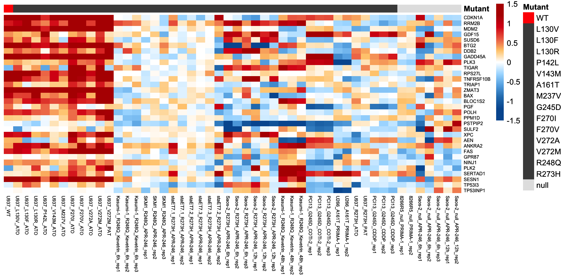
# Visualization of the other 18,264 genes (exclude the 32 confident p53 targets)
plot.mat <- compare.mat[!rownames(compare.mat) %in% tp53.target.g32, ]
p <- pheatmap(plot.mat, scale = "none",
              color = my.colors, breaks = my.breaks,
              cluster_row = F, cluster_col = F, border_color = NA,
              annotation_col = anno.data,
              annotation_colors = anno.color,
              clustering_method = "ward.D2",
              clustering_distance_rows = "manhattan",
              clustering_distance_cols = "manhattan",
              fontsize_col = 6,
              fontsize_row = 0.1)
p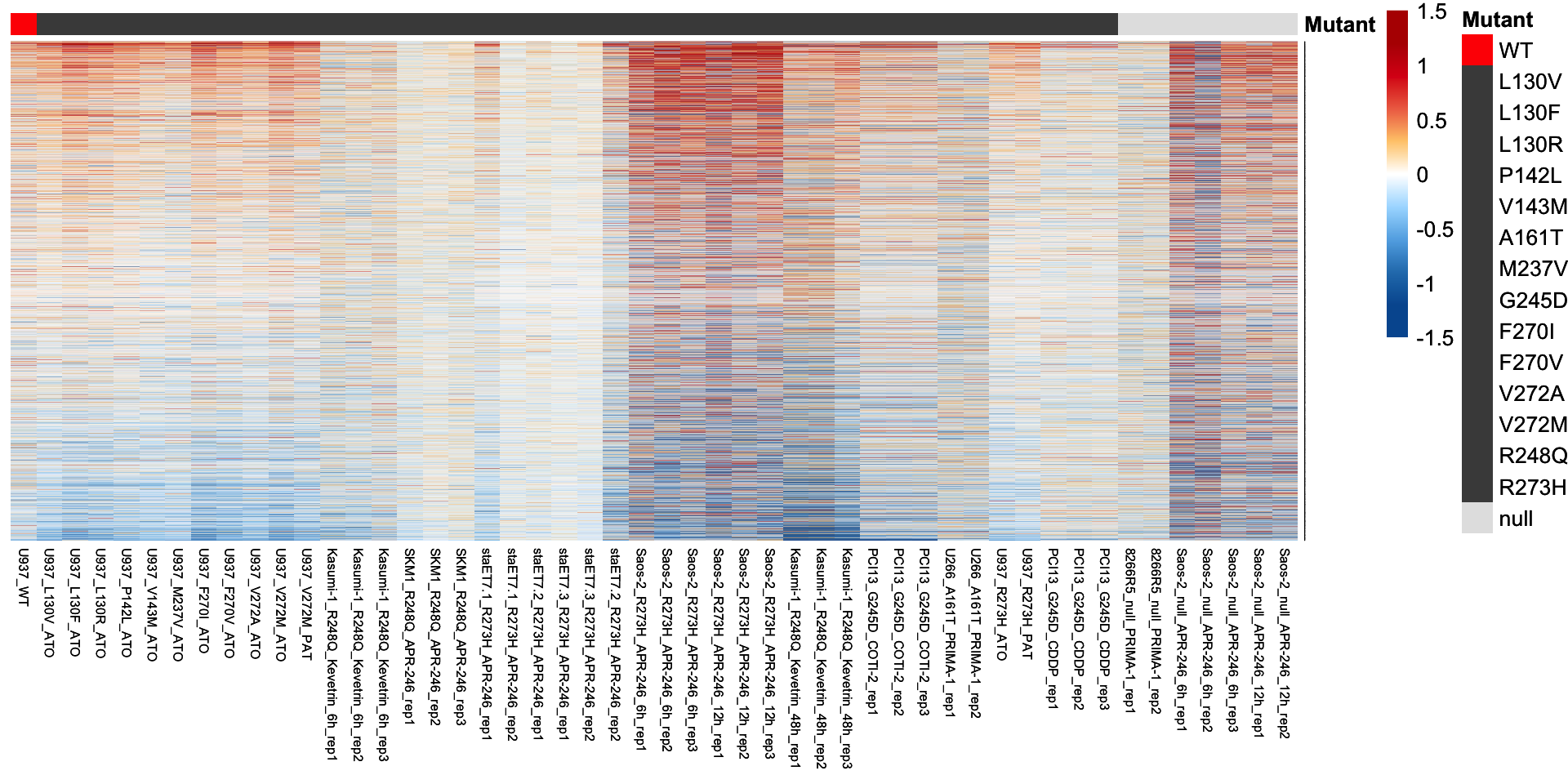
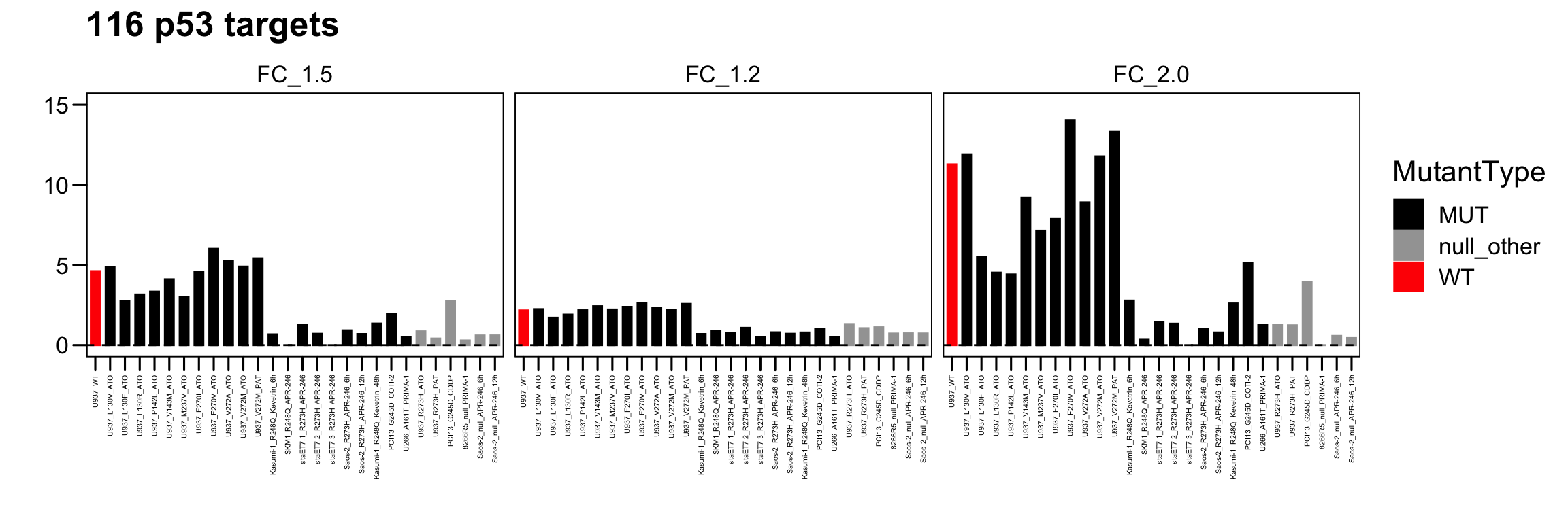
3.5 116 p53 targets
The heatmap plot was used for visualization of the log2-transformed fold change of the 116 p53 targets.
my.breaks <- c(seq(-1.5, -0.01, by = 0.001), seq(0.01, 1.5, by = 0.001) )
my.colors <- c(colorRampPalette(colors = c("#00599F","#00599F","#287dba","#62aee5","#a8dcff","white"))(length(my.breaks)/2),
               colorRampPalette(colors = c("white","#ffca79","#ef6e51","#db1b18","#b50600","#b50600"))(length(my.breaks)/2))

plot.mat <- compare.mat[tp53.target.g116, ]
anno.data <- data.frame(row.names = merge.compare.data$Sample, Mutant = merge.compare.data$p53.status)

# Visualization of the 116 p53 targets
p <- pheatmap(plot.mat, scale = "none",
              color = my.colors, breaks = my.breaks,
              cluster_row = F, cluster_col = F, border_color = NA,
              annotation_col = anno.data,
              annotation_colors = anno.color,
              clustering_method = "ward.D2",
              clustering_distance_rows = "manhattan",
              clustering_distance_cols = "manhattan",
              fontsize_col = 6,
              fontsize_row = 2)
p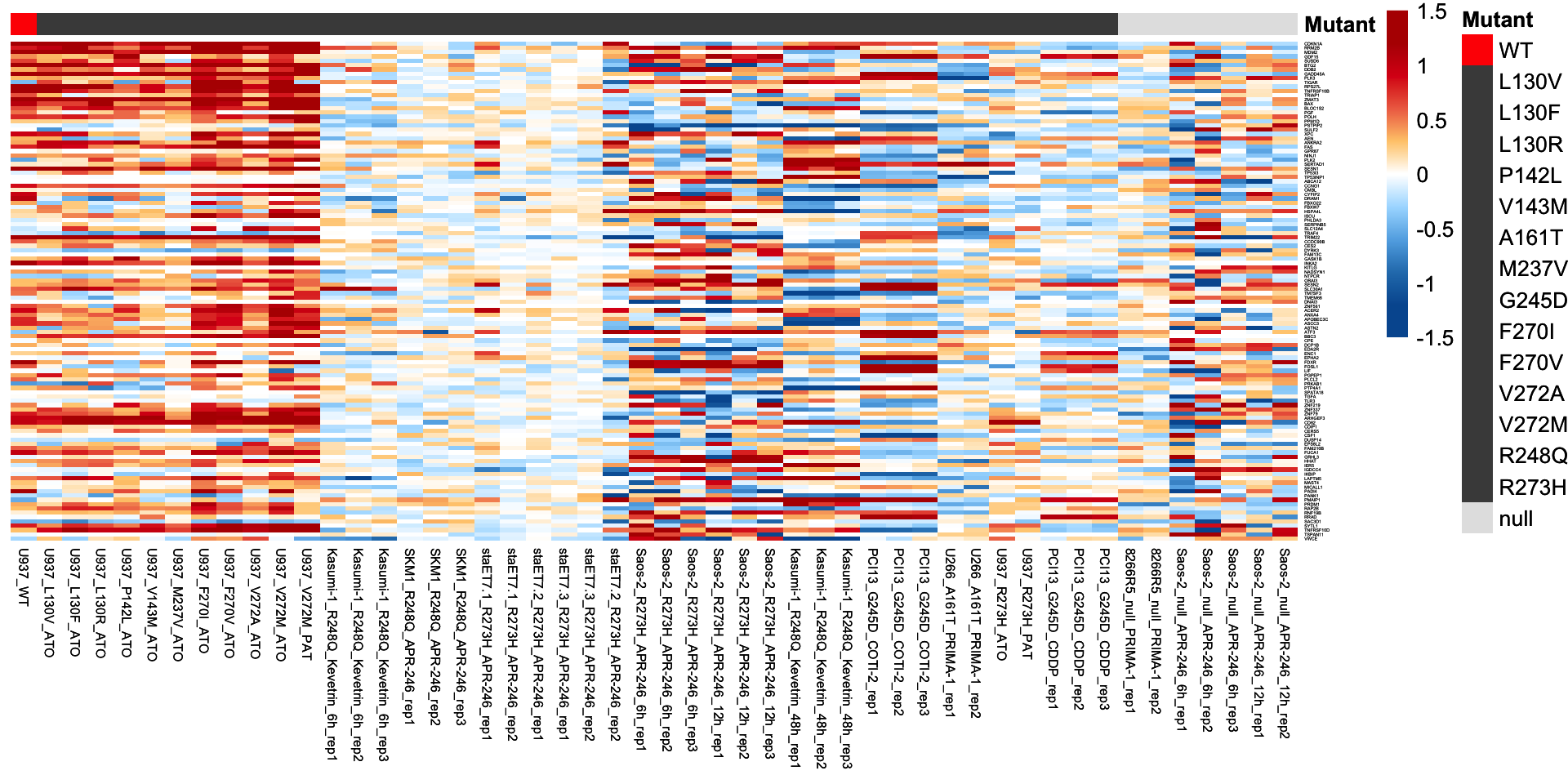
# Visualization of the other 18,180 genes (exclude the 116 p53 targets)
plot.mat <- compare.mat[!rownames(compare.mat) %in% tp53.target.g116, ]
p <- pheatmap(plot.mat, scale = "none",
              color = my.colors, breaks = my.breaks,
              cluster_row = F, cluster_col = F, border_color = NA,
              annotation_col = anno.data,
              annotation_colors = anno.color,
              clustering_method = "ward.D2",
              clustering_distance_rows = "manhattan",
              clustering_distance_cols = "manhattan",
              fontsize_col = 8,
              fontsize_row = 0.1)
p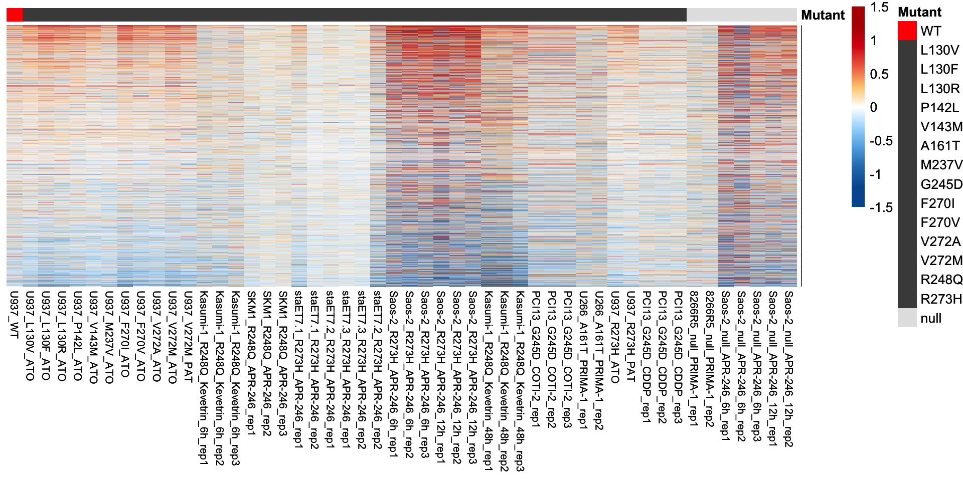
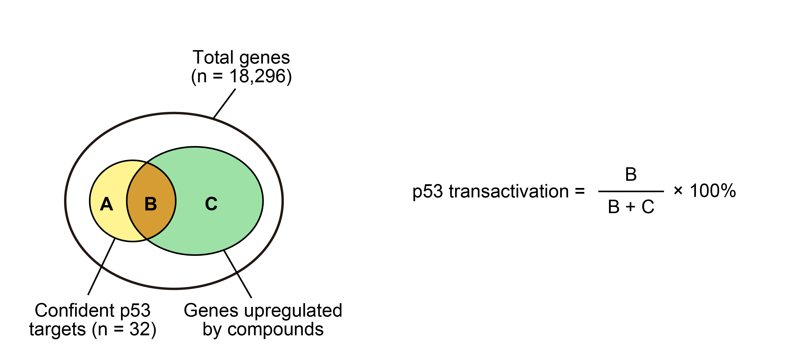
3.6 p53 transactivation
plot.order <- c("U937_WT","U937_L130V_ATO","U937_L130F_ATO","U937_L130R_ATO","U937_P142L_ATO","U937_V143M_ATO","U937_M237V_ATO","U937_F270I_ATO","U937_F270V_ATO","U937_V272A_ATO","U937_V272M_ATO","U937_V272M_PAT","Kasumi-1_R248Q_Kevetrin_6h","SKM1_R248Q_APR-246","staET7.1_R273H_APR-246","staET7.2_R273H_APR-246","staET7.3_R273H_APR-246","Saos-2_R273H_APR-246_6h","Saos-2_R273H_APR-246_12h","Kasumi-1_R248Q_Kevetrin_48h","PCI13_G245D_COTI-2","U266_A161T_PRIMA-1","U937_R273H_ATO","U937_R273H_PAT","PCI13_G245D_CDDP","8266R5_null_PRIMA-1","Saos-2_null_APR-246_6h","Saos-2_null_APR-246_12h")

total.act <- NULL
total.test.cutoff <- c(1.2, 1.5, 2.0)

for (i in 1:length(total.test.cutoff)) {

  cutoff_tmp <- round(log2(total.test.cutoff[i]), 2)
  plot.data <- data.frame(Sample = colnames(compare.mat),
                          UP_116 = colSums(compare.mat[tp53.target.g116, ] > cutoff_tmp) ,
                          UP_32 = colSums(compare.mat[tp53.target.g32, ] > cutoff_tmp),
                          UP_other_116 = colSums(compare.mat[!rownames(compare.mat) %in% tp53.target.g116, ] > cutoff_tmp) ,
                          UP_other_32 = colSums(compare.mat[!rownames(compare.mat) %in% tp53.target.g32, ] > cutoff_tmp) )
  plot.data$Mutant <- merge.compare.data$p53.status[match(plot.data$Sample, merge.compare.data$Sample)]
  plot.data$MutantType <- "MUT"
  plot.data$MutantType[which(plot.data$Mutant == "WT")] <- "WT"

  plot.data$Act_32 <- (plot.data$UP_32) / (plot.data$UP_other_32 + plot.data$UP_32) * 100
  plot.data$Act_116 <- (plot.data$UP_116) / (plot.data$UP_other_116 + plot.data$UP_116) * 100
  plot.data$Group <- merge.compare.data$Group[match(plot.data$Sample, merge.compare.data$Sample)]

  plot.data$Act_32[which(is.na(plot.data$Act_32))] = 1
  plot.data$Act_116[which(is.na(plot.data$Act_116))] = 1

  plot.data.group <- aggregate(plot.data[, c("Act_32","Act_116")], list(Sample = plot.data$Group), mean)
  plot.data.group <- plot.data.group[match(plot.order, plot.data.group$Sample), ]
  plot.data.group$Mutant <- merge.compare.data$p53.status[match(plot.data.group$Sample, merge.compare.data$Group)]
  plot.data.group$MutantType <- "MUT"
  plot.data.group$MutantType[which(plot.data.group$Mutant == "null")] <- "null_other"
  plot.data.group$MutantType[which(plot.data.group$Sample %in% c("U937_R273H_ATO","U937_R273H_PAT","PCI13_G245D_CDDP"))] <- "null_other"
  plot.data.group$MutantType[which(plot.data.group$Mutant == "WT")] <- "WT"

  if (cutoff_tmp != 1) {
    group.tag <- paste0("FC_", total.test.cutoff[i] )
  } else {
    group.tag <- "FC_2.0"
  }

  plot.data.group$Group <- group.tag

  total.act <- rbind(total.act, plot.data.group)
}

total.act$Group <- factor(as.character(total.act$Group), levels = c("FC_1.5","FC_1.2","FC_2.0"))

p <- ggbarplot(total.act, x = "Sample", y = "Act_32",
               color = "MutantType", fill = "MutantType",
               sorting = "none", size = 0.5,
               order = plot.order,
               main = paste0("32 confident p53 targets"), xlab = "", ylab = "",
               palette = c("black","#A3A3A3","red"), width = 0.6 ) + theme_few()
p <- p + geom_hline(yintercept = 0, linetype = 2, color = "black")
p <- p + theme_base() + theme(axis.text.x = element_text(angle = 90, hjust = 1, vjust = 0.5, size = 4))
p <- p + theme(plot.background = element_blank())
p <- p + scale_y_continuous(limits = c(0,11) )
p <- p + facet_wrap( ~ Group, ncol = 3)
p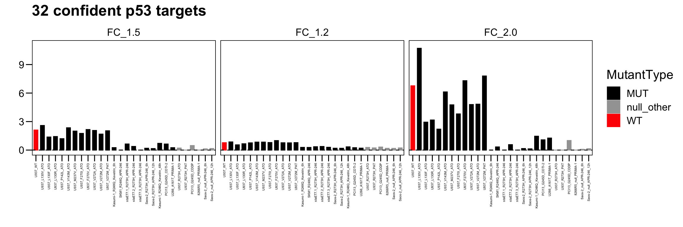
p <- ggbarplot(total.act, x = "Sample", y = "Act_116",
               color = "MutantType", fill = "MutantType",
               sorting = "none", size = 0.5,
               order = plot.order,
               main = paste0("116 p53 targets"), xlab = "", ylab = "",
               palette = c("black","#A3A3A3","red"), width = 0.6 ) + theme_few()
p <- p + geom_hline(yintercept = 0, linetype = 2, color = "black")
p <- p + theme_base() + theme(axis.text.x = element_text(angle = 90, hjust = 1, vjust = 0.5, size = 4))
p <- p + theme(plot.background = element_blank())
p <- p + scale_y_continuous(limits = c(0,15) )
p <- p + facet_wrap( ~ Group, ncol = 3)
p