CTRL_BM
library(Seurat)
library(dplyr)
library(Matrix)
library(gplots)
library(matrixStats)
library(ggpubr)
library(openxlsx)
library(stringr)
library(ggthemes)
library(pheatmap)
library(SingleR)
library(monocle3) # devtools::install_github('cole-trapnell-lab/monocle3')
library(harmony) # install.packages("harmony")
#----------------------------------------------------------------------------------
# Step 1: setting
#----------------------------------------------------------------------------------
rm(list = ls())
color.lib <- c("#E31A1C", "#55c2fc", "#A6761D", "#F1E404", "#33A02C", "#1F78B4",
"#FB9A99", "#FDBF6F", "#FF7F00", "#CAB2D6", "#6A3D9A", "#F4B3BE",
"#1B9E77", "#D95F02", "#7570B3", "#E7298A", "#66A61E", "#E6AB02",
"#F4A11D", "#8DC8ED", "#4C6CB0", "#8A1C1B", "#CBCC2B", "#EA644C",
"#634795", "#005B1D", "#26418A", "#CB8A93", "#B2DF8A", "#E22826",
"#A6CEE3", "#F4D31D", "#F4A11D", "#82C800", "#8B5900", "#858ED1",
"#FF72E1", "#CB50B2", "#007D9B", "#26418A", "#8B495F", "#FF394B")
sample.name = "CTRL_BM"
message(sample.name)
# Set output path
out.path <- paste0("output/", sample.name) #system(sprintf("mkdir %s", out.path))
dir.create(out.path,recursive = T)
#----------------------------------------------------------------------------------
# Step 2: Setup the Seurat Object
#----------------------------------------------------------------------------------
# load data from data folder
scell.data <- Read10X(data.dir = paste0("data/", sample.name) )
colnames(scell.data) <- str_replace_all(colnames(scell.data), "1", sample.name)
# Initialize the Seurat object with the raw (non-normalized data)
sce <- CreateSeuratObject(counts = scell.data, project = "sce", min.cells = 0, min.features = 0)
# Add sample information
sce@meta.data$Sample = sample.name
sce
head(sce@meta.data)
#----------------------------------------------------------------------------------
# Step 3: QC and selecting cells
#----------------------------------------------------------------------------------
# key challenges: ensure that only single, live cells are included in downstream analysis
## mitochondrial gene
sce[["percent.mt"]] <- PercentageFeatureSet(sce, pattern = "^MT-")
sce
summary(sce@meta.data$percent.mt)
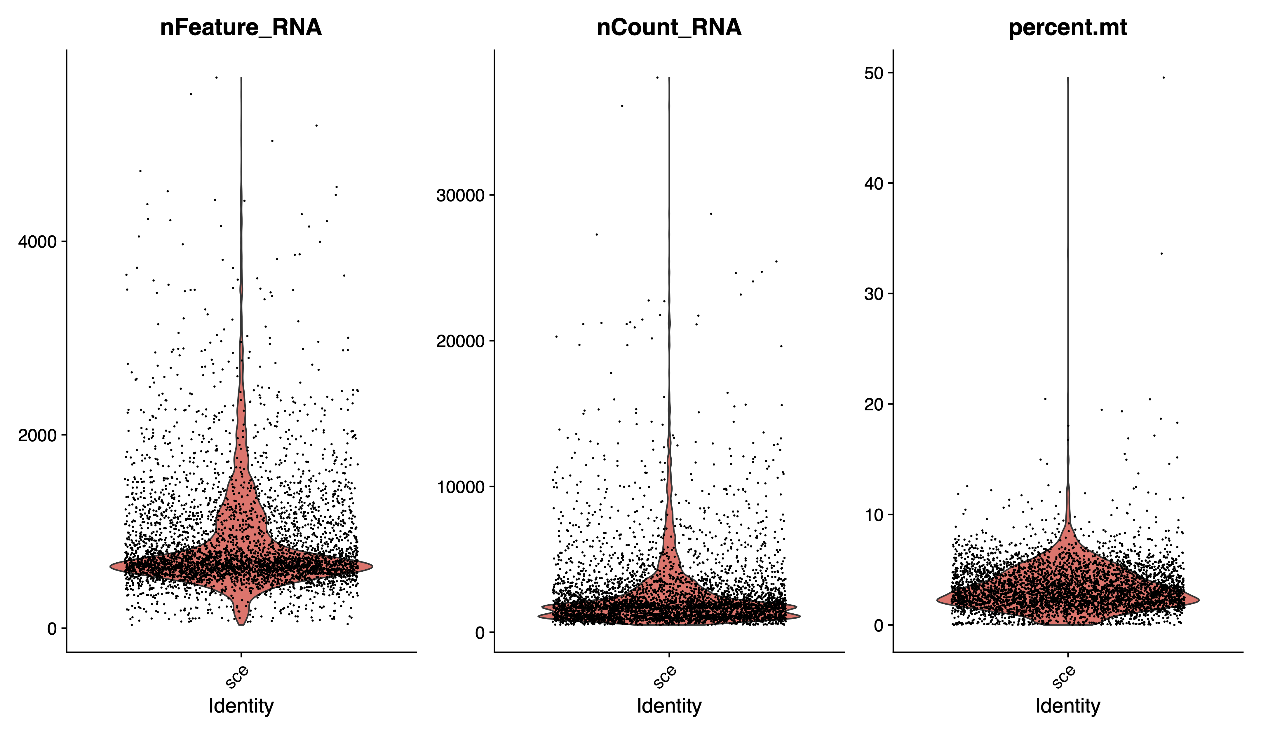
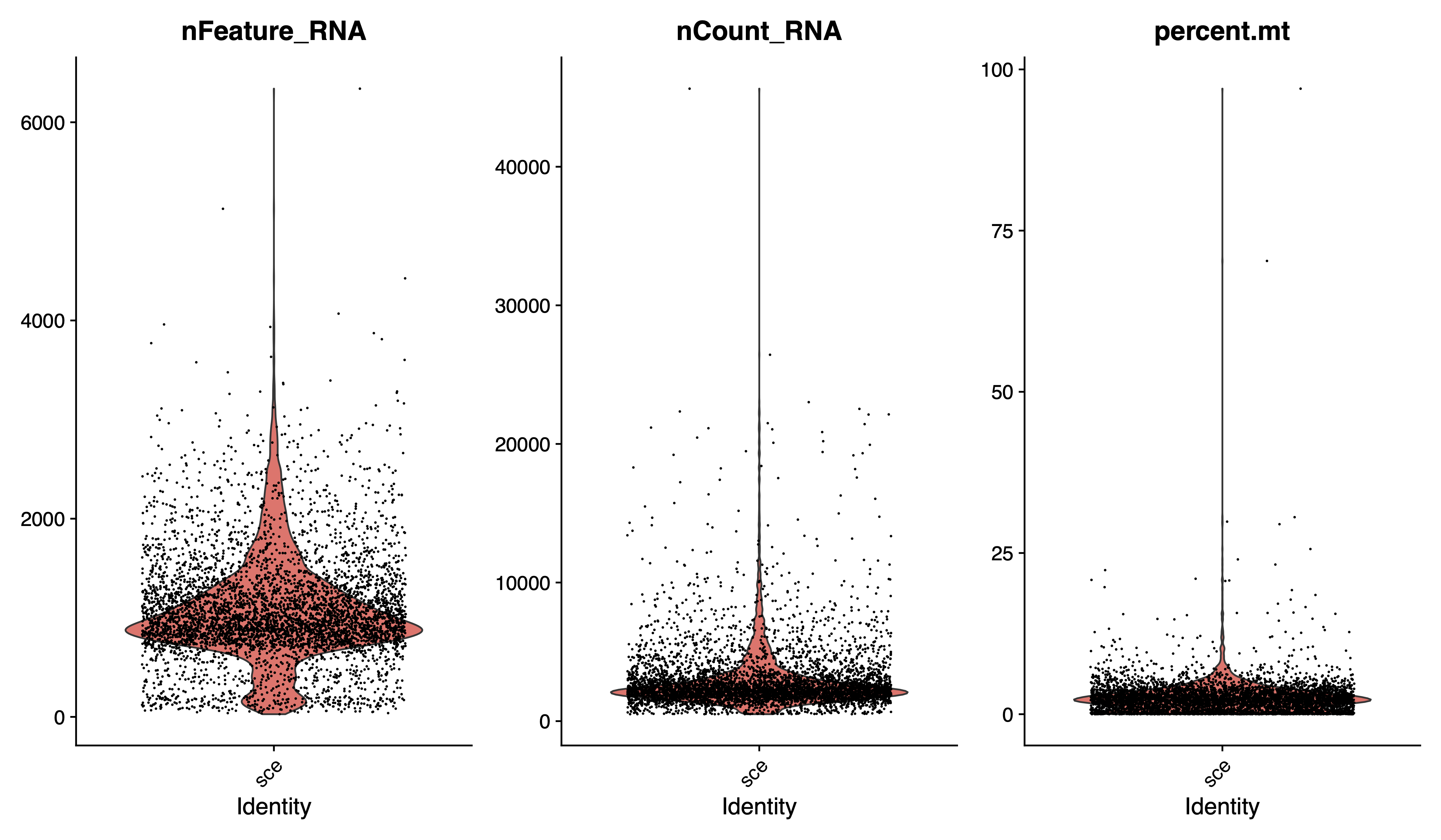
# Visualize QC metrics as a violin plot
pdf(paste0(out.path, "/1.vlnplot.pdf"), width = 12, height = 7)
VlnPlot(sce, features = c("nFeature_RNA", "nCount_RNA", "percent.mt"), group.by = "orig.ident", ncol = 3)
dev.off()
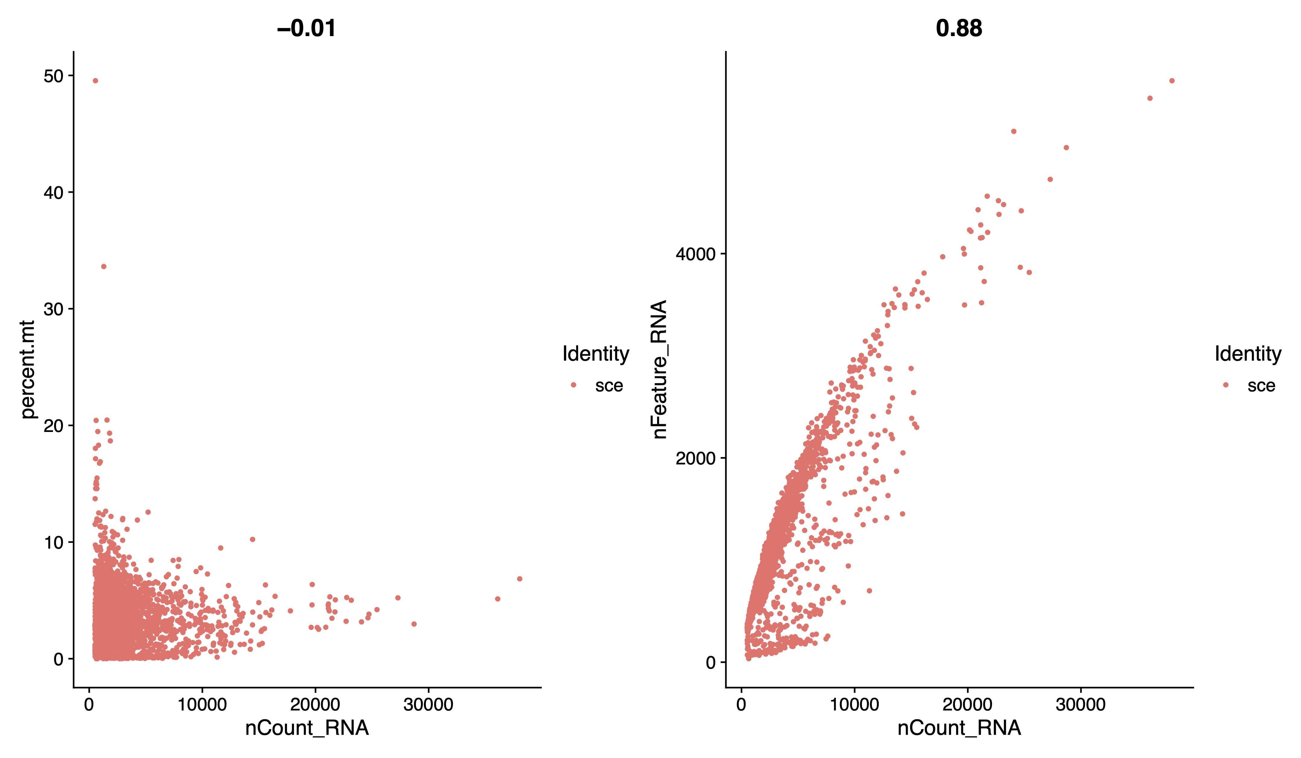
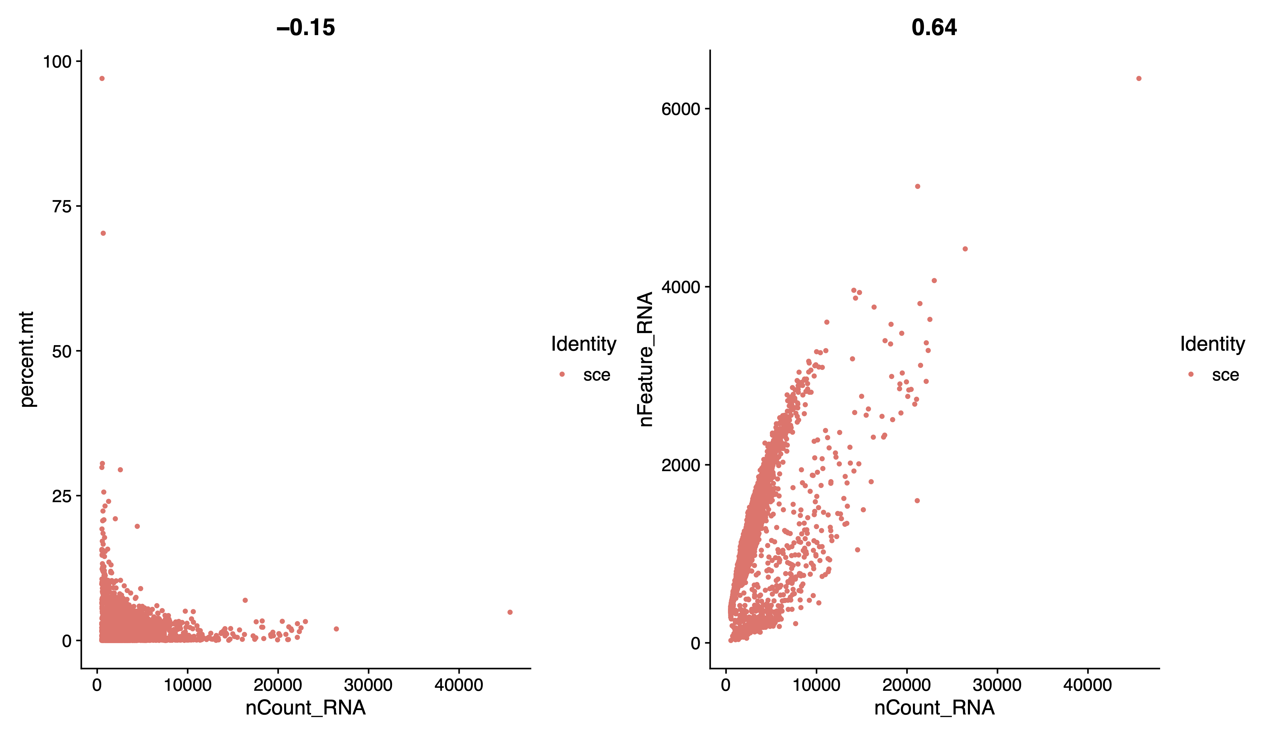
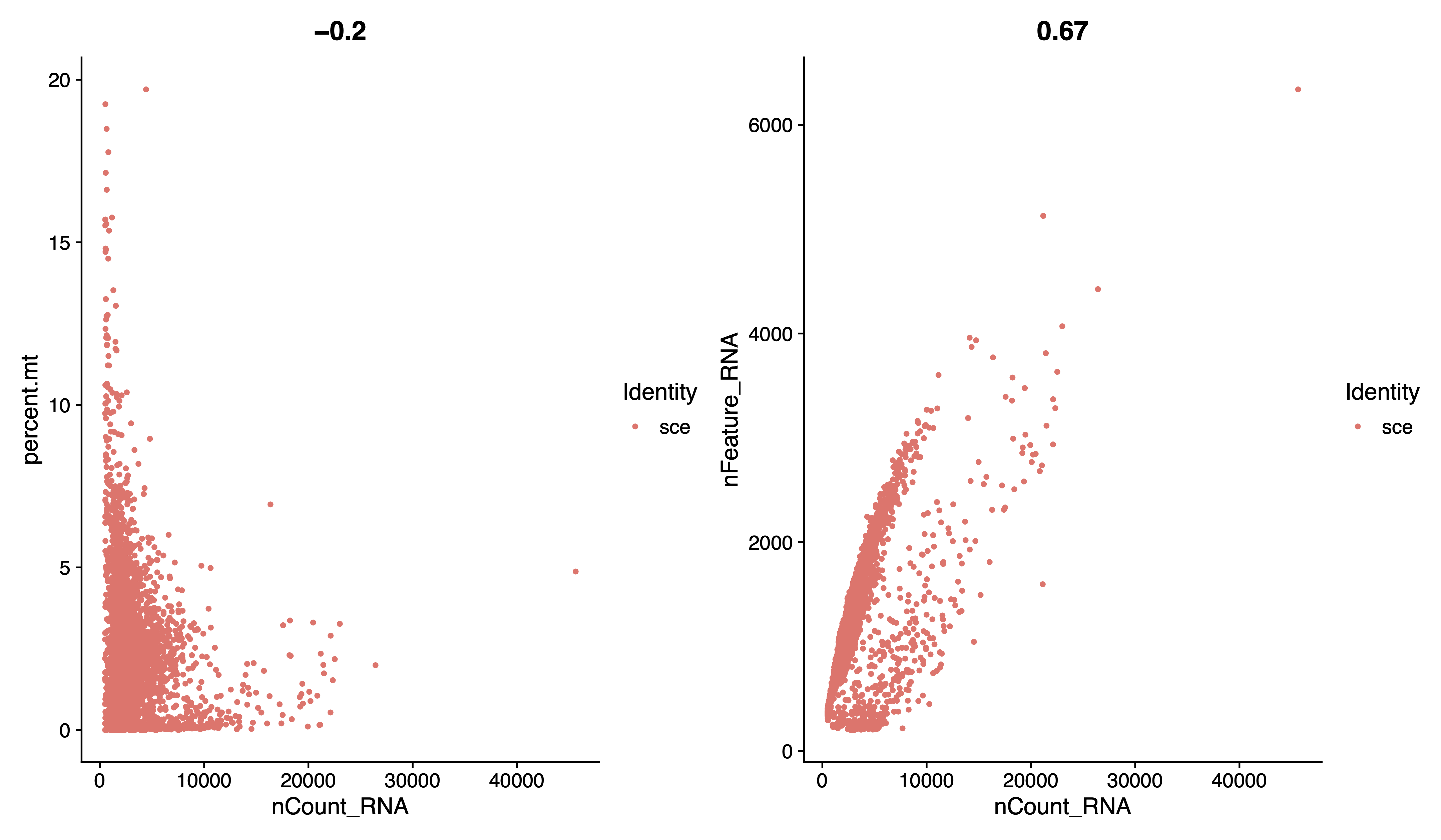
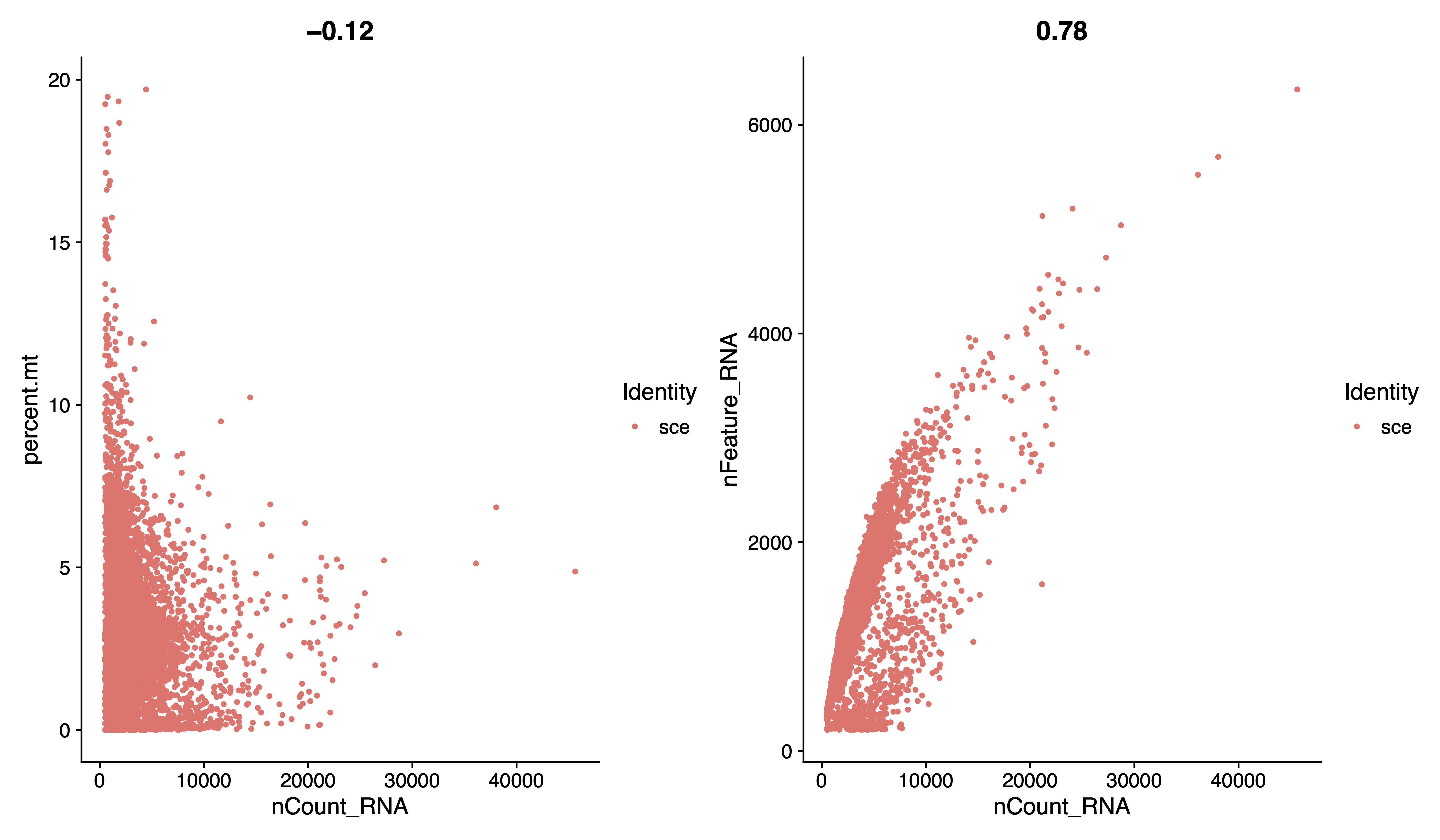
# visualize feature-feature relationships
pdf(paste0(out.path, "/1.geneplot.pdf"), width = 12, height = 7)
plot1 <- FeatureScatter(sce, feature1 = "nCount_RNA", feature2 = "percent.mt")
plot2 <- FeatureScatter(sce, feature1 = "nCount_RNA", feature2 = "nFeature_RNA")
plot1 + plot2
dev.off()
## QC : selecting cells
sce <- subset(sce, subset = nFeature_RNA > 200 & percent.mt < 20)
sce
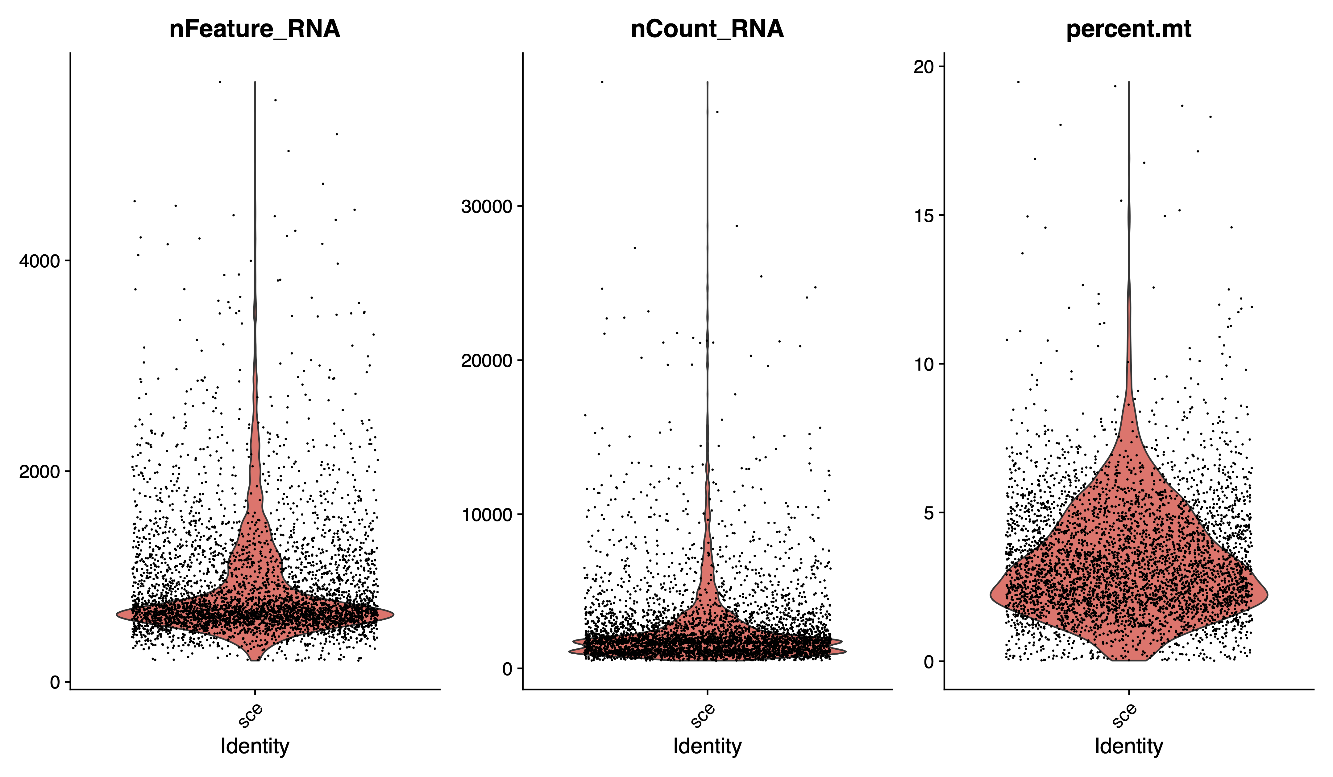
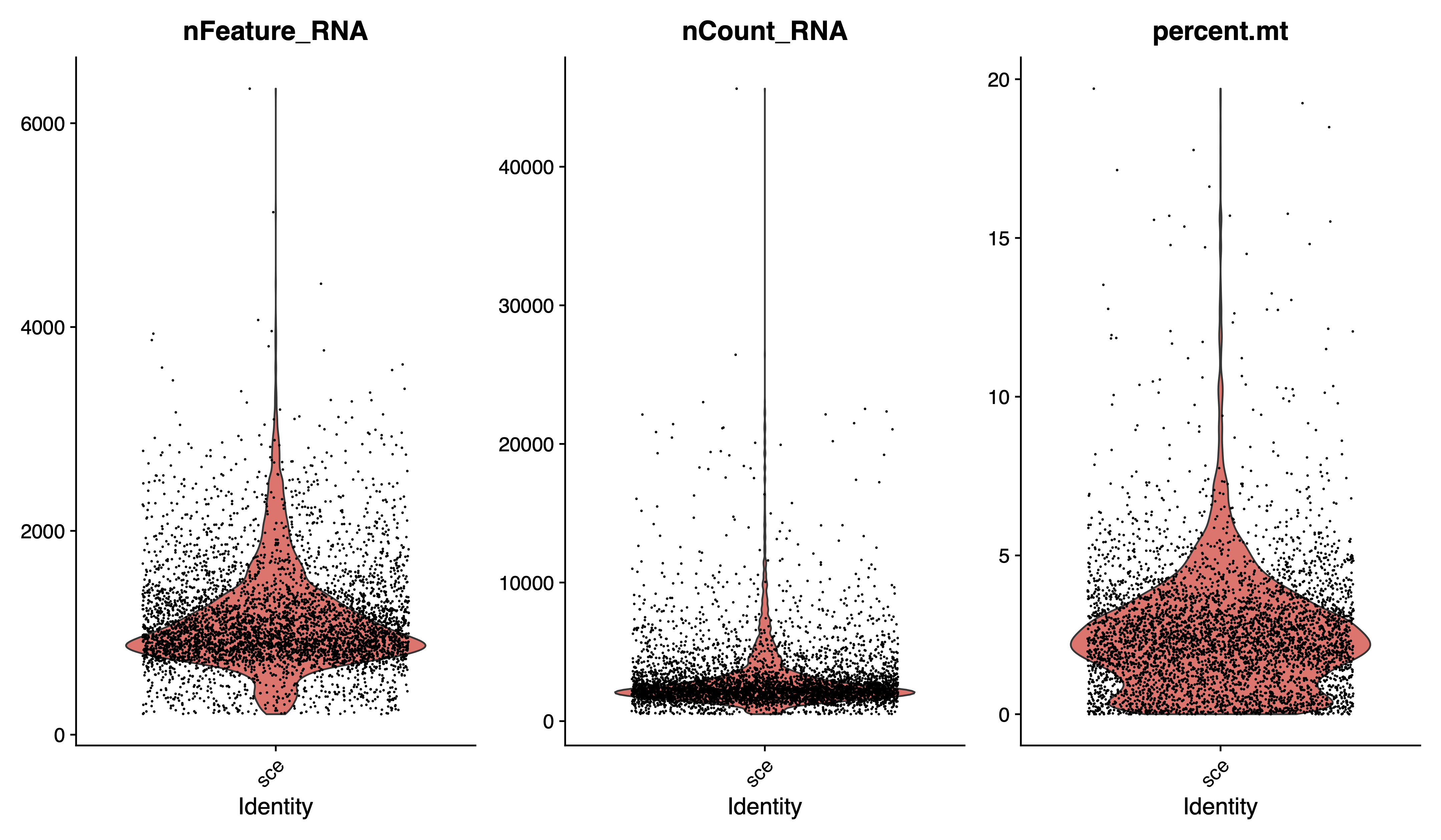
# plot after QC
pdf(paste0(out.path, "/2.filter.vlnplot.pdf"), width = 12, height = 7)
VlnPlot(sce, features = c("nFeature_RNA", "nCount_RNA", "percent.mt"), group.by = "orig.ident", ncol = 3)
dev.off()
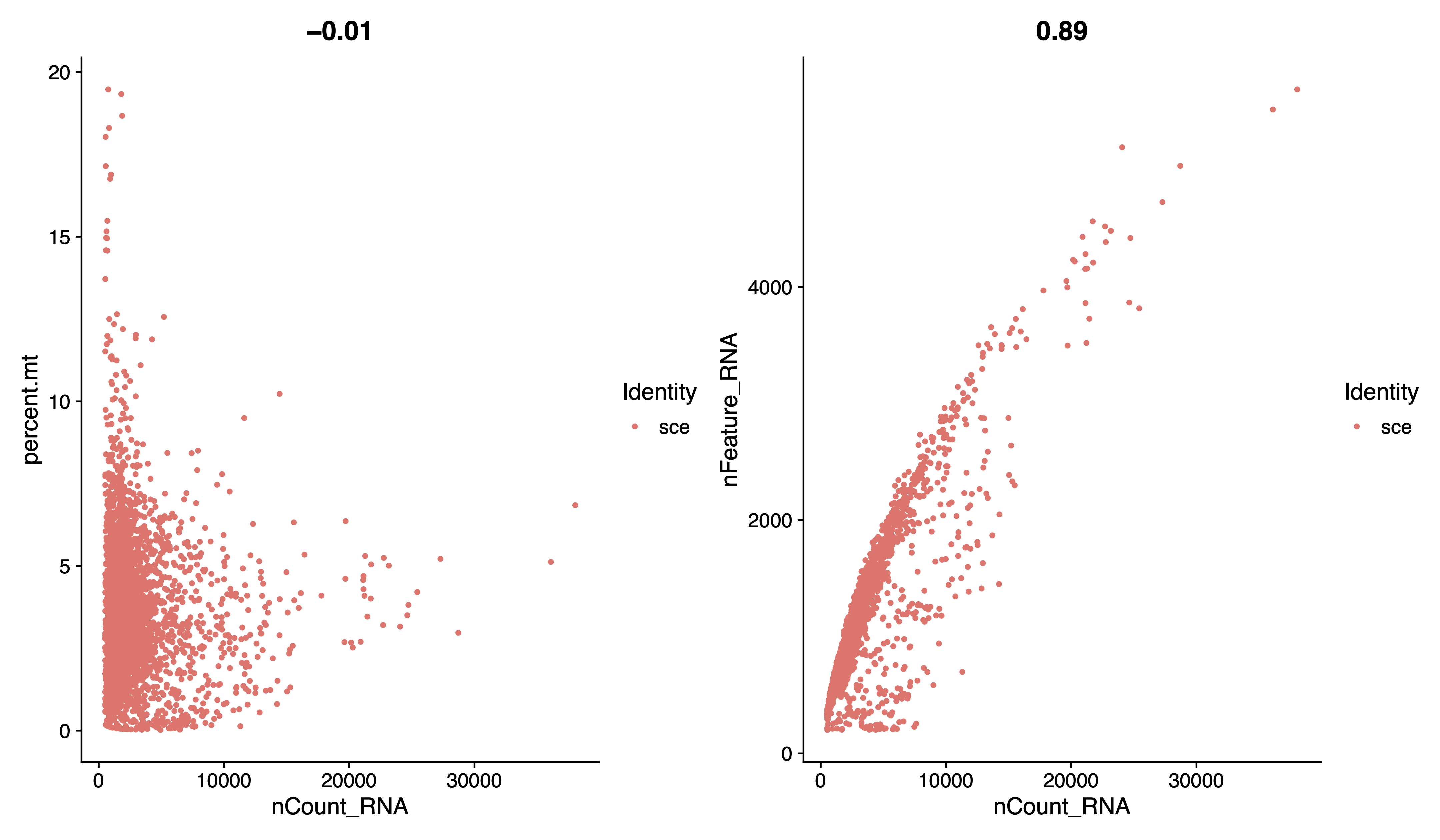
pdf(paste0(out.path, "/2.filter.geneplot.pdf"), width = 12, height = 7)
plot1 <- FeatureScatter(sce, feature1 = "nCount_RNA", feature2 = "percent.mt")
plot2 <- FeatureScatter(sce, feature1 = "nCount_RNA", feature2 = "nFeature_RNA")
plot1 + plot2
dev.off()
#----------------------------------------------------------------------------------
# Step 4: Normalizing the data
#----------------------------------------------------------------------------------
# After removing unwanted cells from the dataset, the next step is to normalize the data.
sce <- NormalizeData(sce, normalization.method = "LogNormalize", scale.factor = ncol(sce))
# By default, we employ a global-scaling normalization method “LogNormalize” that normalizes the feature expression measurements for each cell by the total expression, multiplies this by a scale factor (10,000 by default), and log-transforms the result. Normalized values are stored in pbmc[["RNA"]]@data
sce[["RNA"]]@data[1:20,1:5]
#----------------------------------------------------------------------------------
# Step 5: Identification of highly variable features (feature selection)
#----------------------------------------------------------------------------------
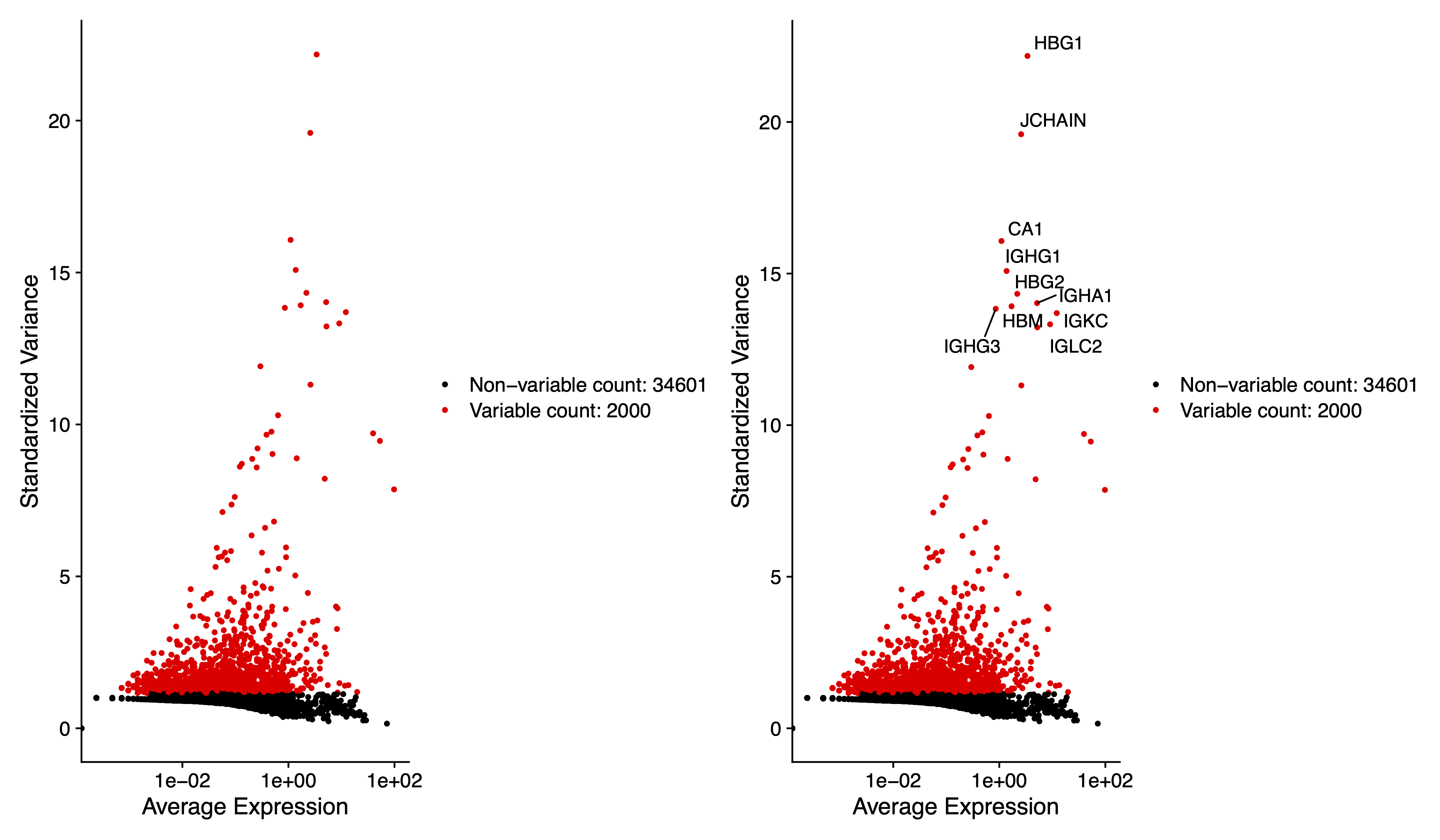
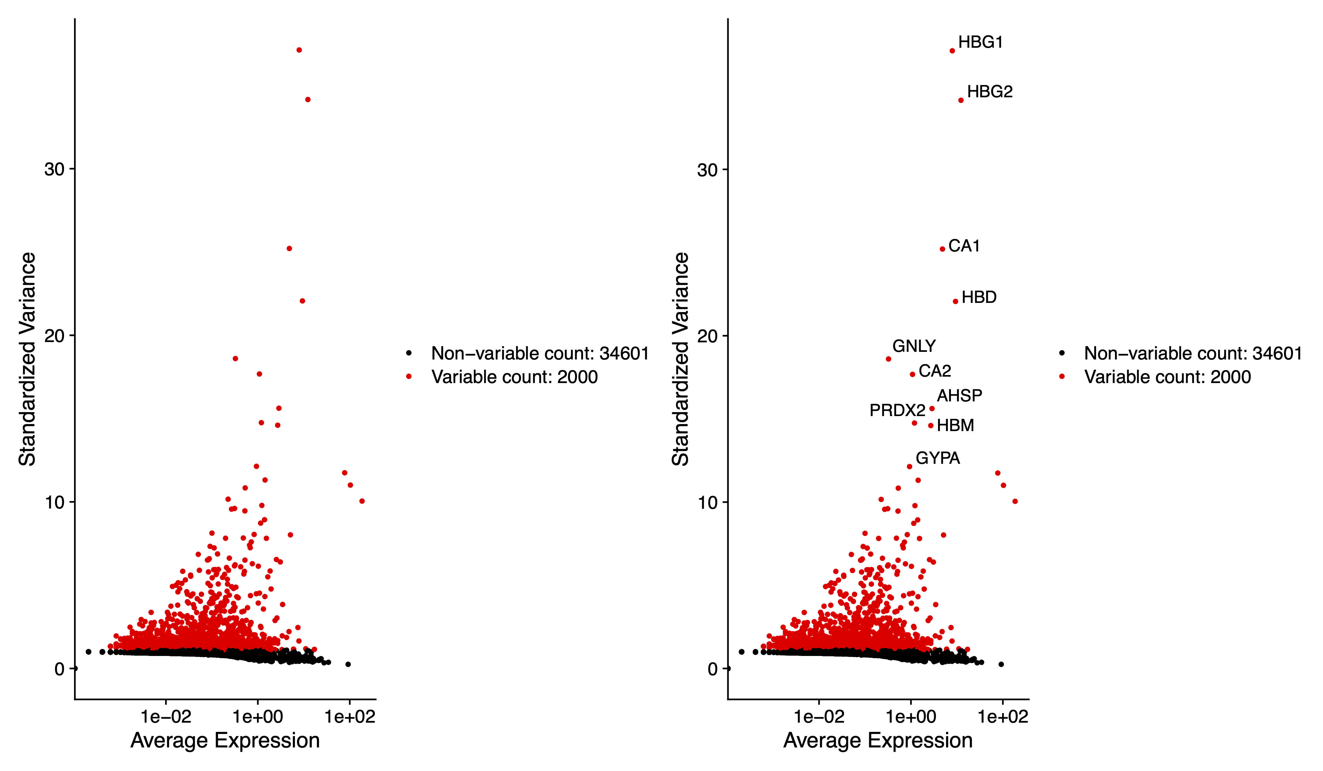
# We next calculate a subset of features that exhibit high cell-to-cell variation in the dataset
sce <- FindVariableFeatures(sce, selection.method = "vst", nfeatures = 2000)
# Identify the 10 most highly variable genes
top10 <- head(VariableFeatures(sce), 10)
# plot variable features with and without labels
pdf(paste0(out.path, "/3.VariableFeaturePlot.pdf"), width = 12, height = 7)
plot1 <- VariableFeaturePlot(sce)
plot2 <- LabelPoints(plot = plot1, points = top10, repel = TRUE)
plot1 + plot2
dev.off()
#----------------------------------------------------------------------------------
# Step 6: Scaling the data
#----------------------------------------------------------------------------------
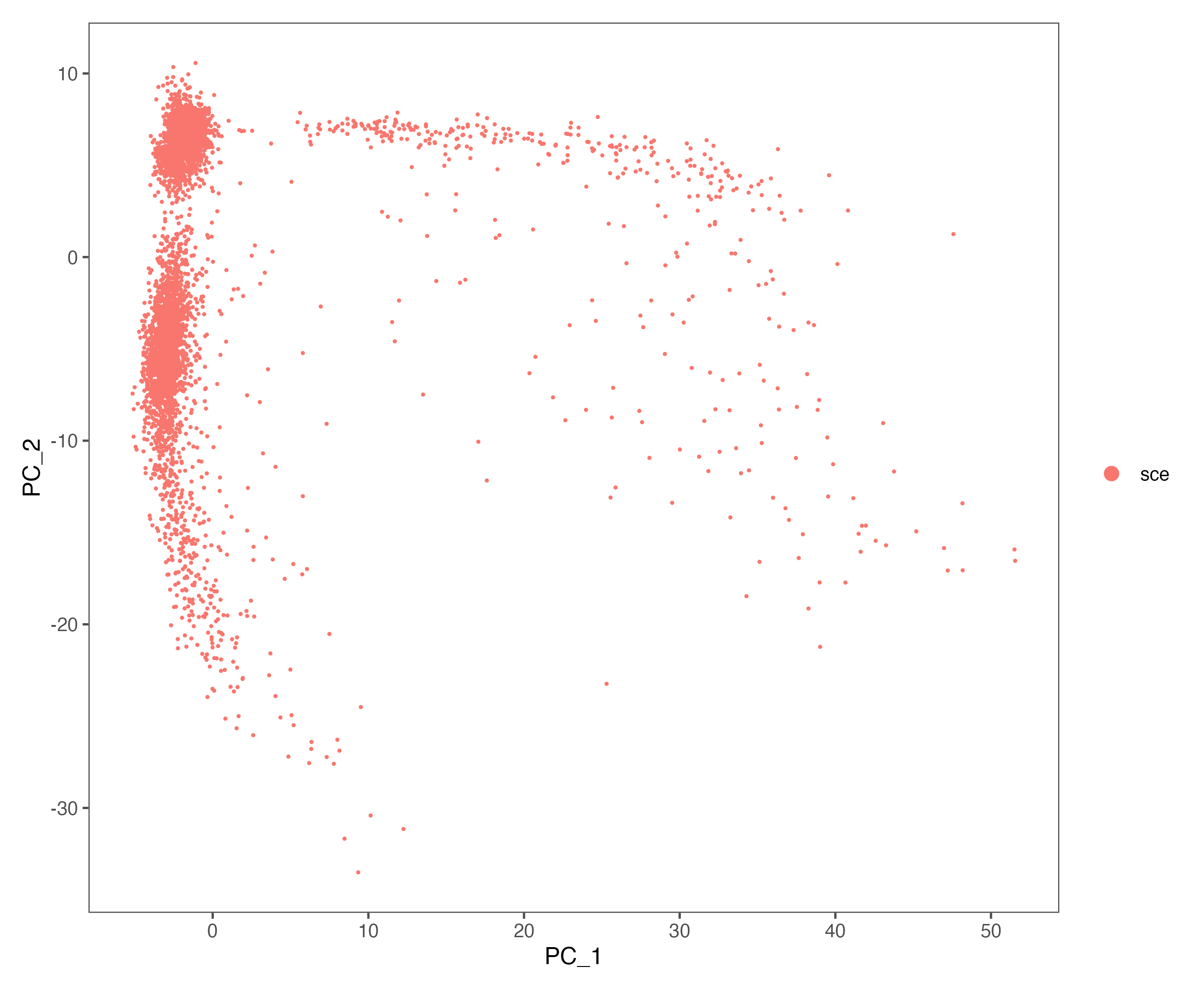
# linear transformation: pre-processing step prior to dimensional reduction techniques like PCA
all.genes <- rownames(sce)
sce <- ScaleData(sce, features = VariableFeatures(sce))
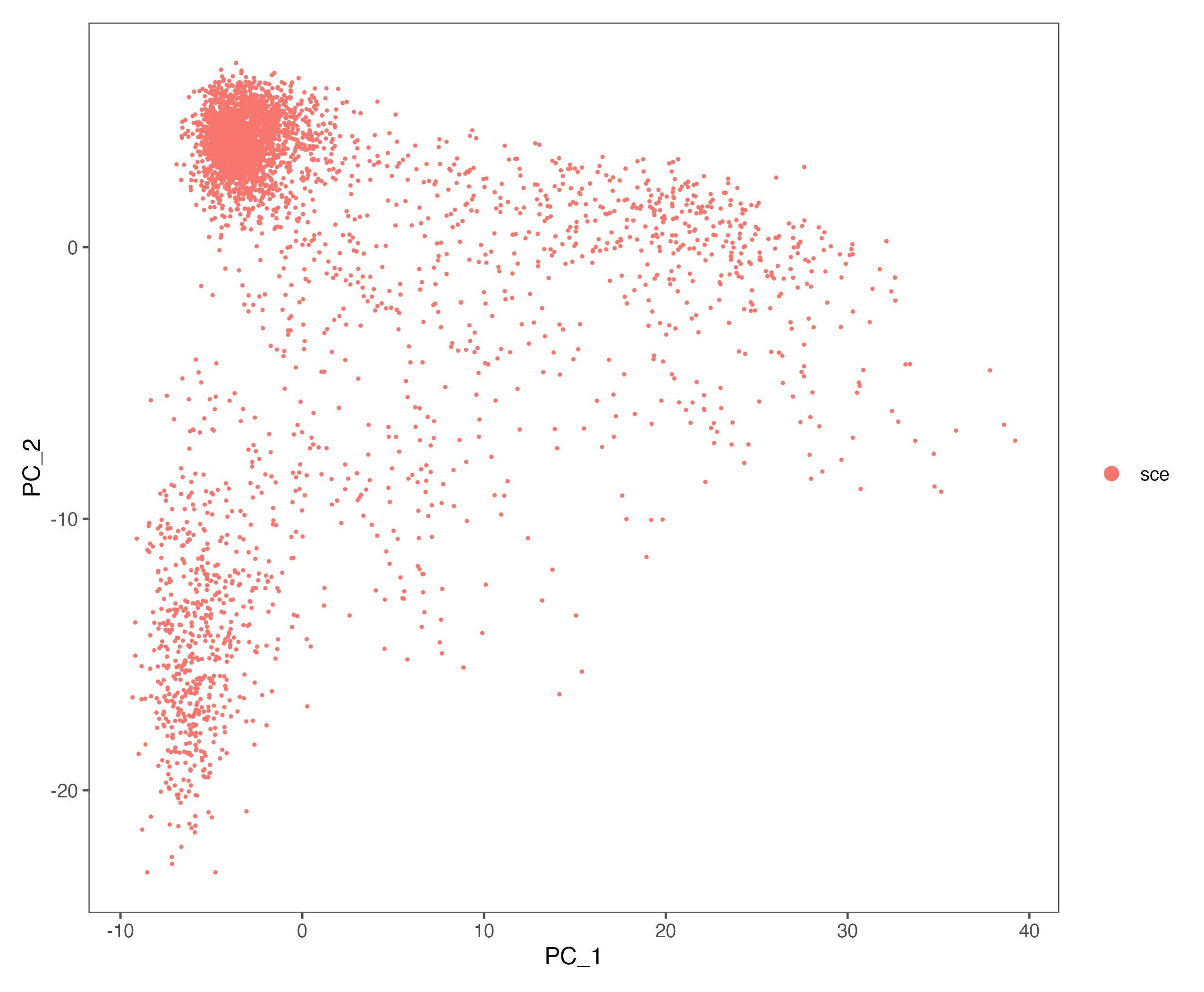
sce <- RunPCA(sce, features = VariableFeatures(object = sce))
p <- DimPlot(sce, reduction = "pca") + theme_few()
ggsave(paste0(out.path, "/4.PCA.pdf"), p, width = 8.5, height = 7)
#----------------------------------------------------------------------------------
# Step 7: Cluster the cells
#----------------------------------------------------------------------------------
sce <- FindNeighbors(sce, reduction = "pca", dims = 1:20)
sce <- FindClusters(sce, resolution = 0.8)
#----------------------------------------------------------------------------------
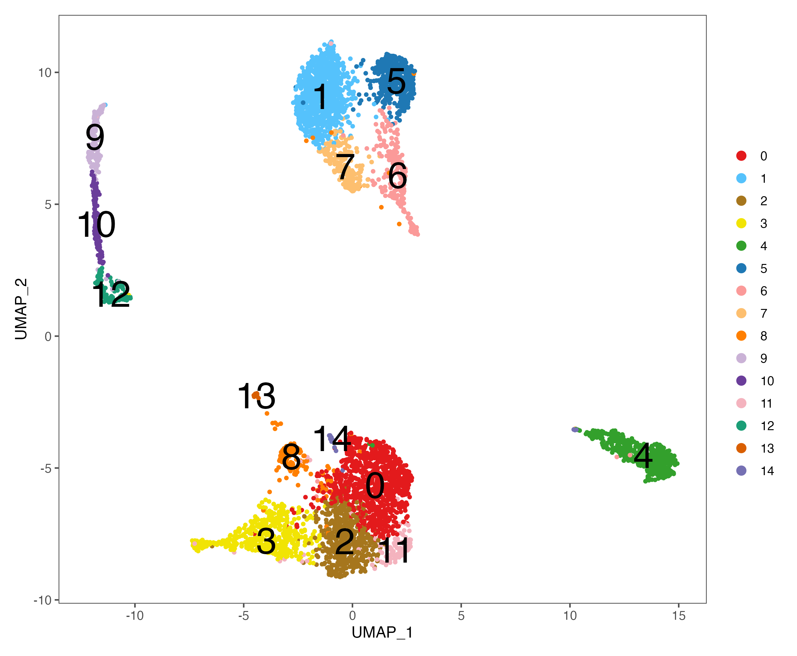
# Step 8: Run non-linear dimensional reduction (UMAP/tSNE)
#----------------------------------------------------------------------------------
# to learn the underlying manifold of the data in order to place similar cells together in low-dimensional space
# If you haven't installed UMAP, you can do so via reticulate::py_install(packages =
# 'umap-learn')
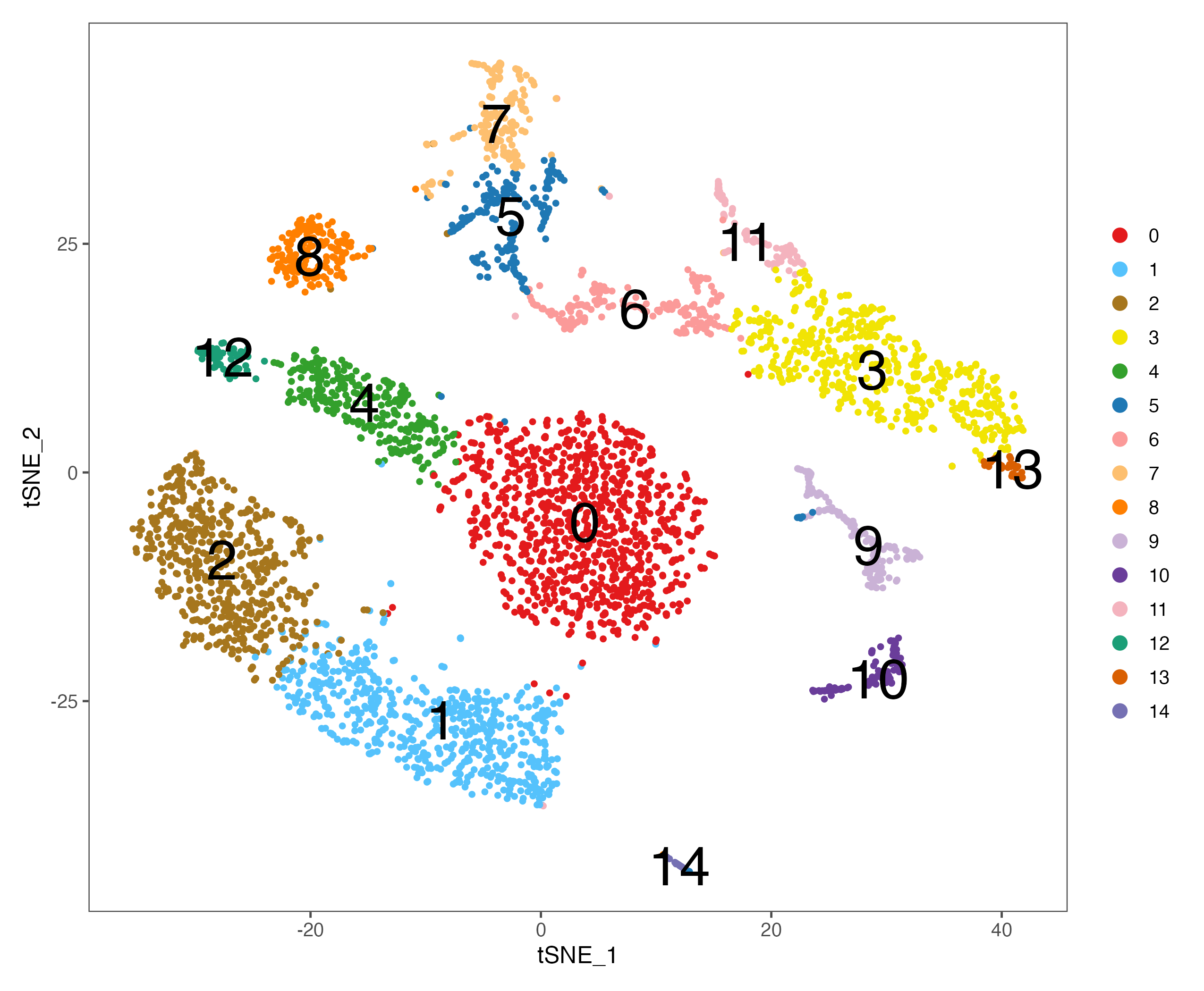
sce <- RunTSNE(sce, reduction = "pca", dims = 1:20, perplexity = 30)
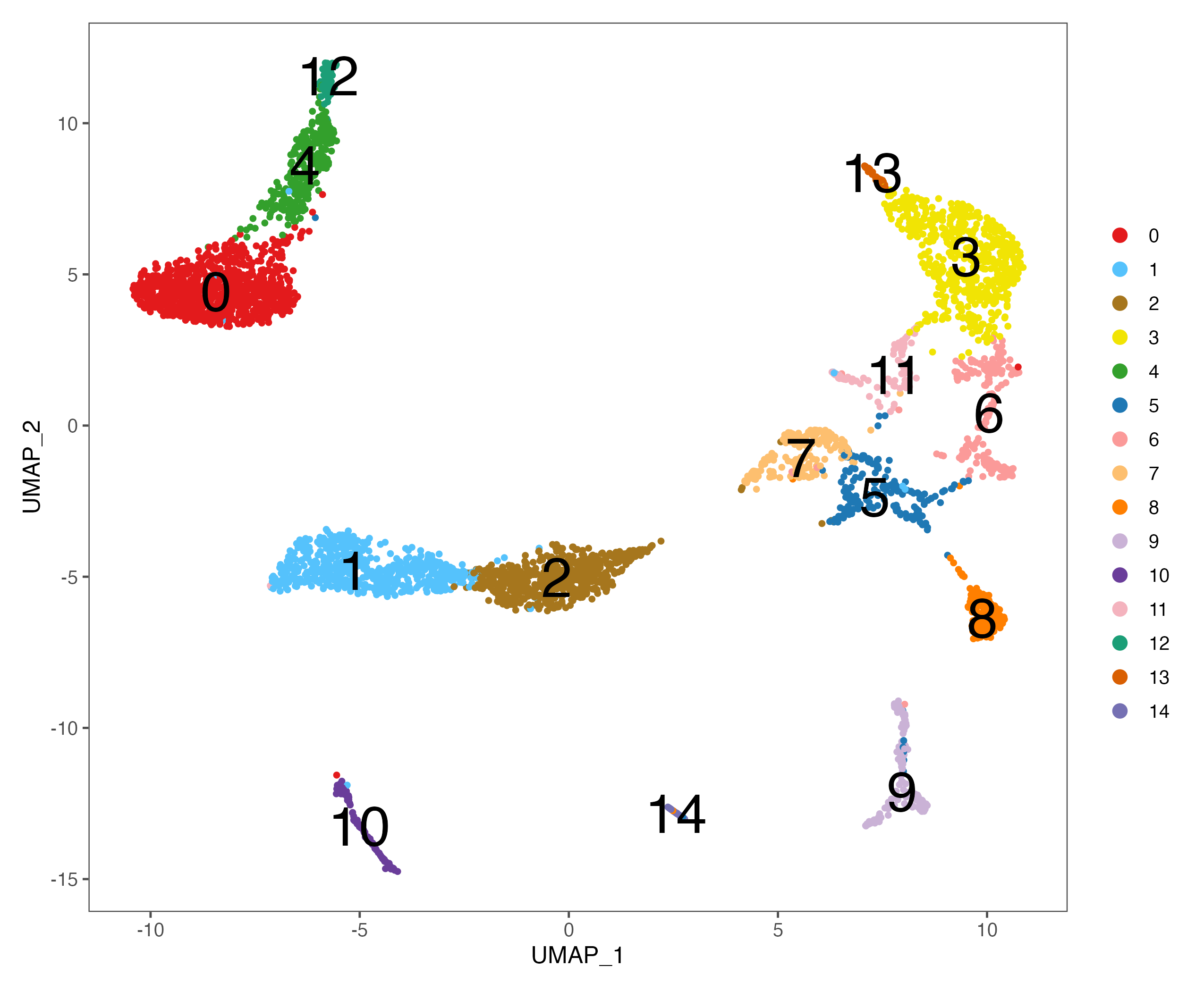
sce <- RunUMAP(sce, reduction = "pca", dims = 1:20)
# plot
# umap
p <- DimPlot(sce, reduction = "umap", pt.size = 1,
cols = color.lib) + theme_few()
ggsave(paste0(out.path, "/5.UMAP.cluster.pdf"), p, width = 8.5, height = 7)
p <- DimPlot(sce, reduction = "umap", pt.size = 1, label = TRUE, label.size = 10,
cols = color.lib) + theme_few()
ggsave(paste0(out.path, "/5.UMAP.cluster.label.pdf"), p, width = 8.5, height = 7)
# tsne
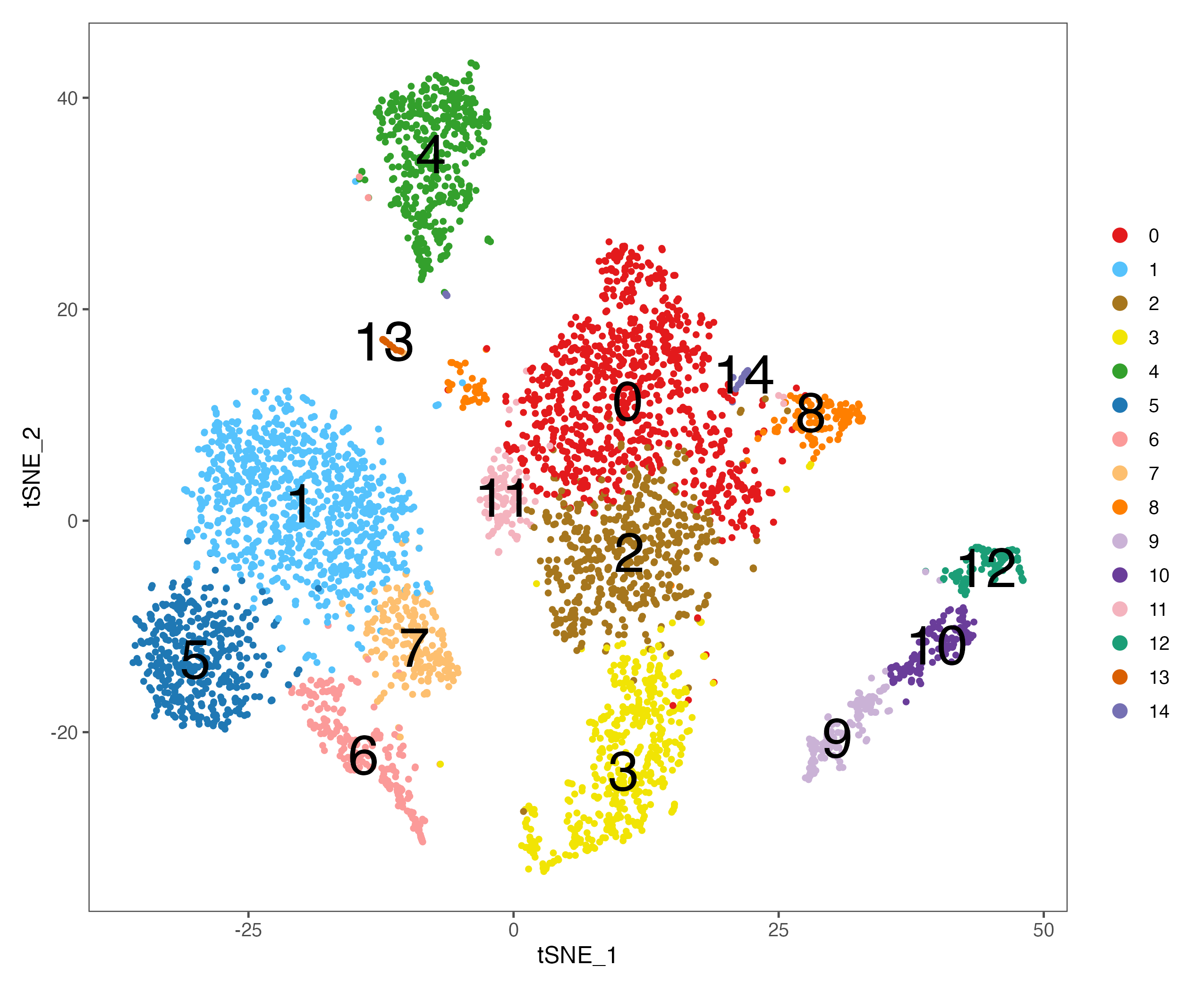
p <- DimPlot(sce, reduction = "tsne", pt.size = 1,
cols = color.lib) + theme_few()
ggsave(paste0(out.path, "/6.tSNE.cluster.pdf"), p, width = 8.5, height = 7)
p <- DimPlot(sce, reduction = "tsne", pt.size = 1, label = TRUE, label.size = 10,
cols = color.lib) + theme_few()
ggsave(paste0(out.path, "/6.tSNE.cluster.label.pdf"), p, width = 8.5, height = 7)
#----------------------------------------------------------------------------------
# Step 9: Cell cycle
#----------------------------------------------------------------------------------
# build-in cell cycle genes
cc.genes
sce <- CellCycleScoring(sce, s.features = cc.genes$s.genes, g2m.features = cc.genes$g2m.genes)
p <- DimPlot(sce, reduction = "umap", pt.size = 1, label = FALSE,
group.by = "Phase", cols = color.lib) + theme_few()
ggsave(paste0(out.path, "/7.CC.phase.pdf"), p, width = 8.5, height = 7)
p <- VlnPlot(sce, features = "S.Score", pt.size = 0,
group.by = "seurat_clusters", cols = color.lib) + theme_few()
ggsave(paste0(out.path, "/7.CC.score.S.Score.pdf"), p, width = 10, height = 5)
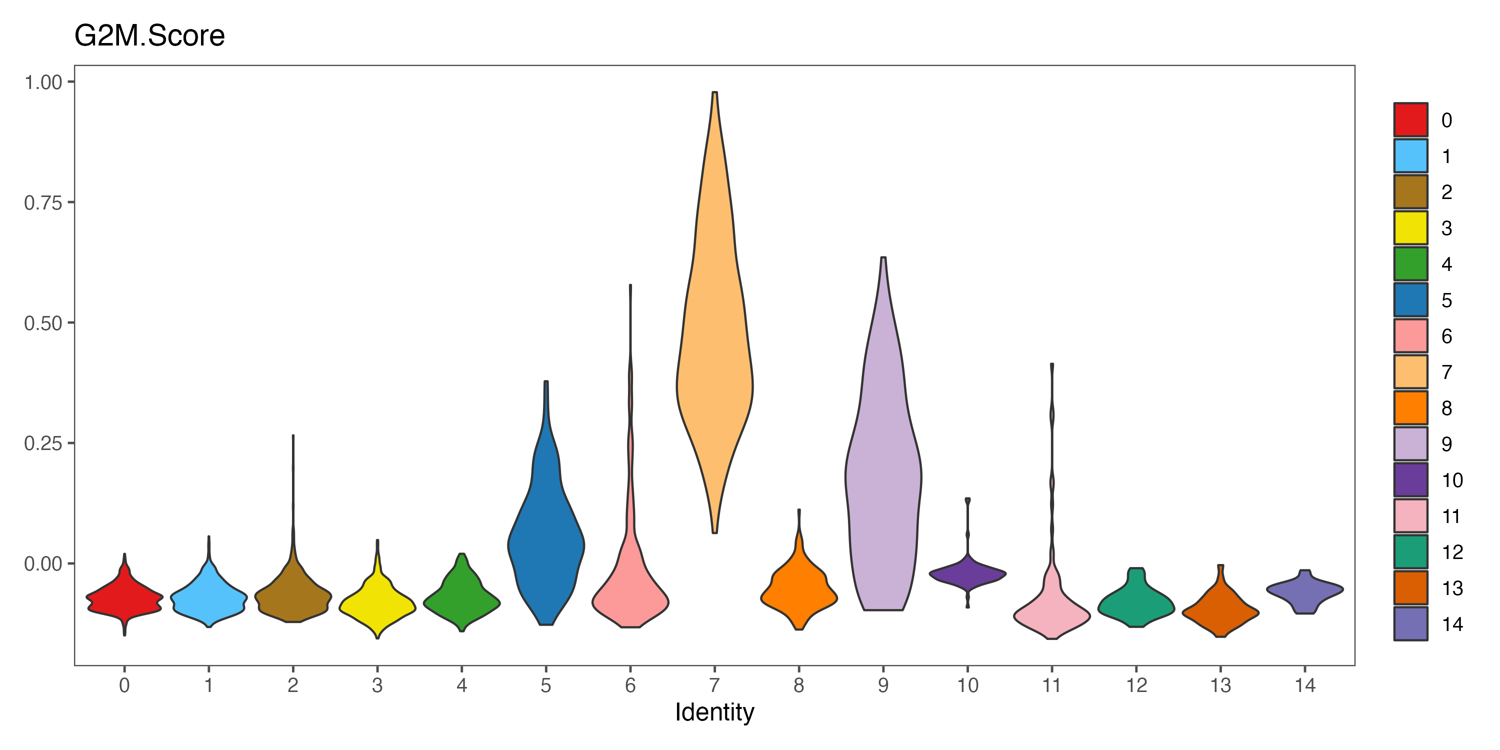
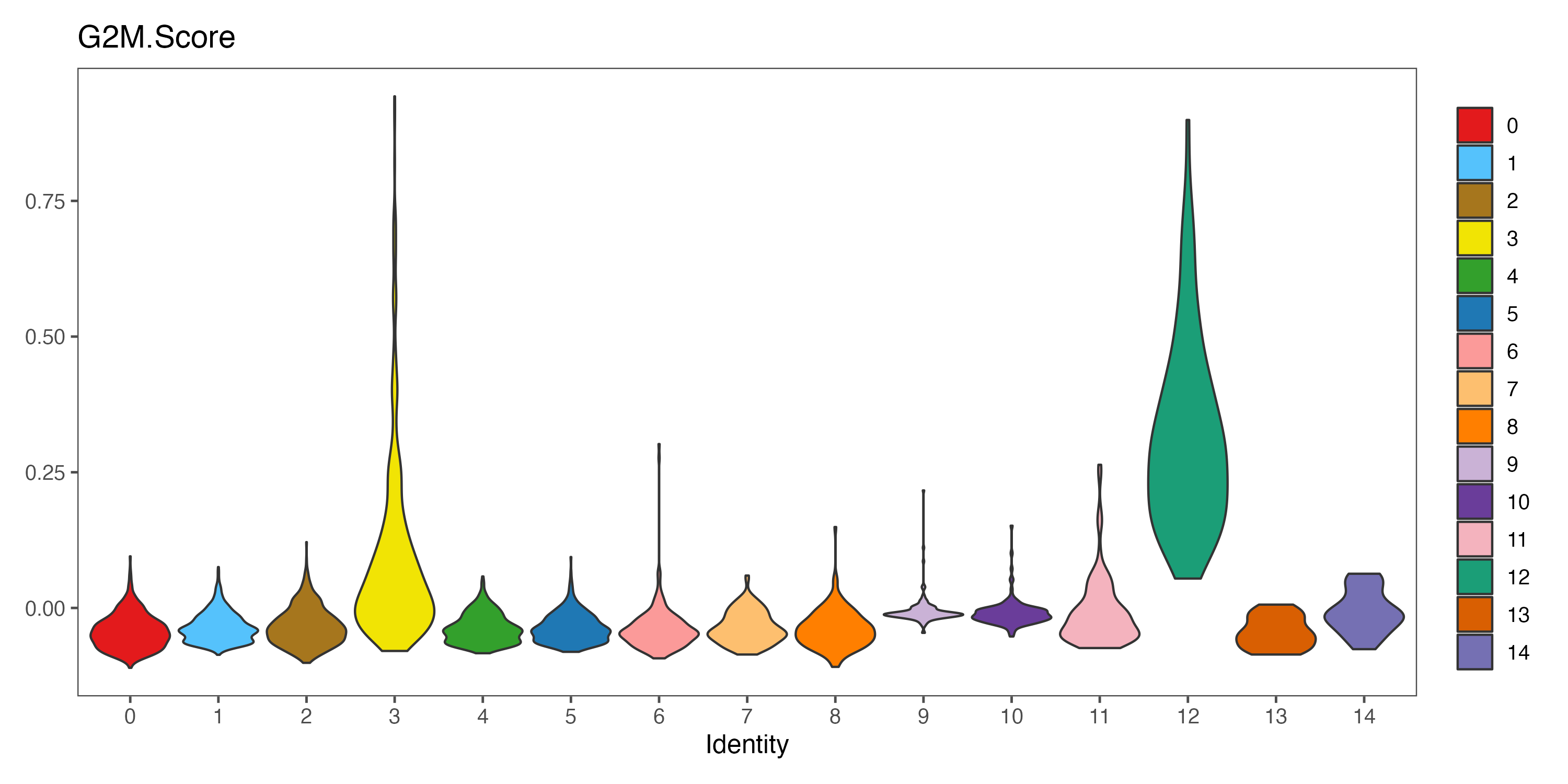
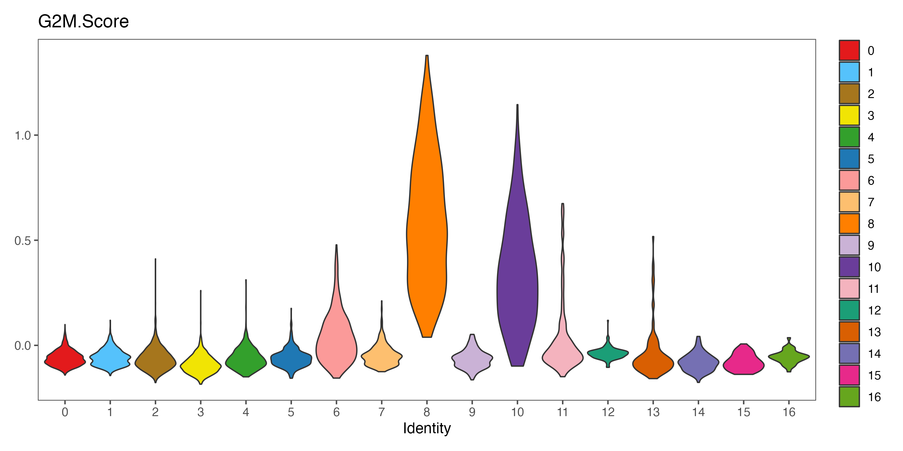
p <- VlnPlot(sce, features = "G2M.Score", pt.size = 0,
group.by = "seurat_clusters", cols = color.lib) + theme_few()
ggsave(paste0(out.path, "/7.CC.score.G2M.Score.pdf"), p, width = 10, height = 5)
#----------------------------------------------------------------------------------
# Step 10: SingleR annotation
#----------------------------------------------------------------------------------
# first, load reference datasets. Then, annotate your query data based on reference datasets.
ref <- readRDS(file = "./data/SingleR/hs.BlueprintEncodeData.RDS")
pred.BlueprintEncodeData <- SingleR(test = sce@assays$RNA@data, ref = ref, labels = ref$label.main)
ref <- readRDS(file = "./data/SingleR/hs.HumanPrimaryCellAtlasData.RDS")
pred.HumanPrimaryCellAtlasData <- SingleR(test = sce@assays$RNA@data, ref = ref, labels = ref$label.main)
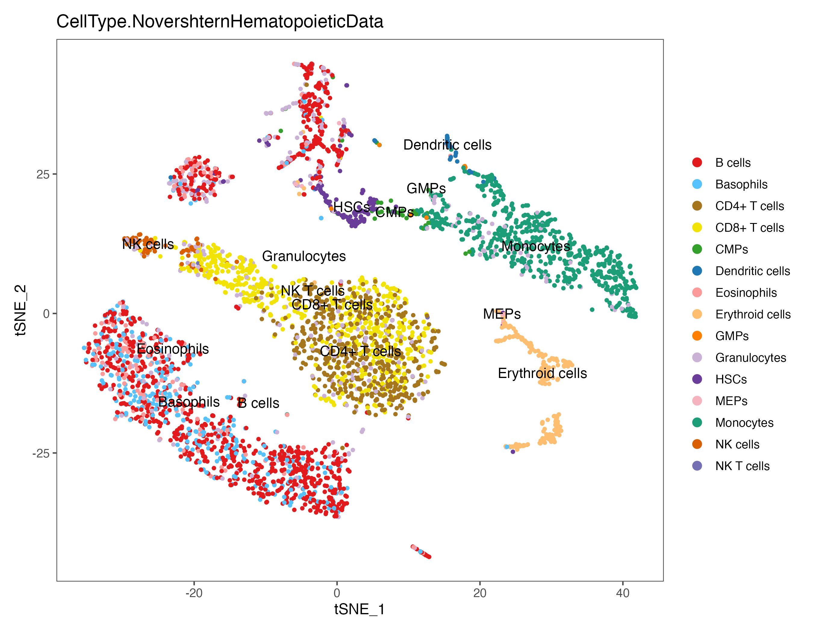
ref <- readRDS(file = "./data/SingleR/NovershternHematopoieticData.RDS")
pred.NovershternHematopoieticData <- SingleR(test = sce@assays$RNA@data, ref = ref, labels = ref$label.main)
# add annotations to meta data
sce@meta.data$CellType.BlueprintEncodeData <- pred.BlueprintEncodeData$labels
sce@meta.data$CellType.HumanPrimaryCellAtlasData <- pred.HumanPrimaryCellAtlasData$labels
sce@meta.data$CellType.NovershternHematopoieticData <- pred.NovershternHematopoieticData$labels
# plot with annotations
# umap
p <- DimPlot(sce, reduction = "umap", pt.size = 1, label = TRUE, label.size = 4,
group.by = "CellType.BlueprintEncodeData", cols = color.lib) + theme_few()
ggsave(paste0(out.path, "/8.SingleR.umap.BlueprintEncodeData.pdf"), p, width = 9, height = 7)
p <- DimPlot(sce, reduction = "umap", pt.size = 1, label = TRUE, label.size = 4,
group.by = "CellType.HumanPrimaryCellAtlasData", cols = color.lib) + theme_few()
ggsave(paste0(out.path, "/8.SingleR.umap.HumanPrimaryCellAtlasData.pdf"), p, width = 9, height = 7)
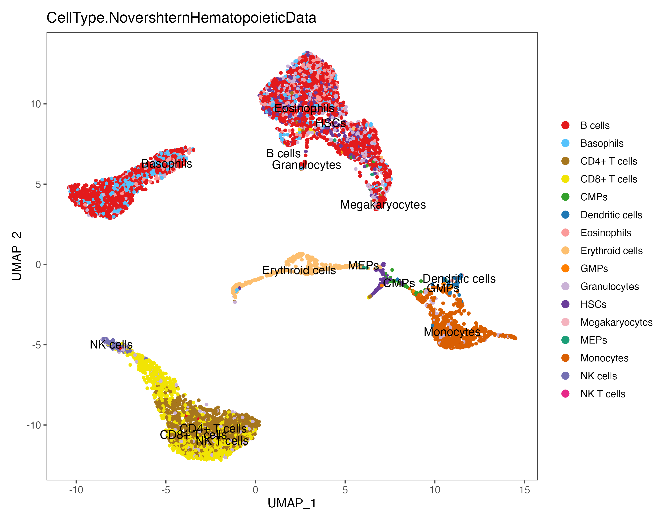
p <- DimPlot(sce, reduction = "umap", pt.size = 1, label = TRUE, label.size = 4,
group.by = "CellType.NovershternHematopoieticData", cols = color.lib) + theme_few()
ggsave(paste0(out.path, "/8.SingleR.umap.NovershternHematopoieticData.pdf"), p, width = 9, height = 7)
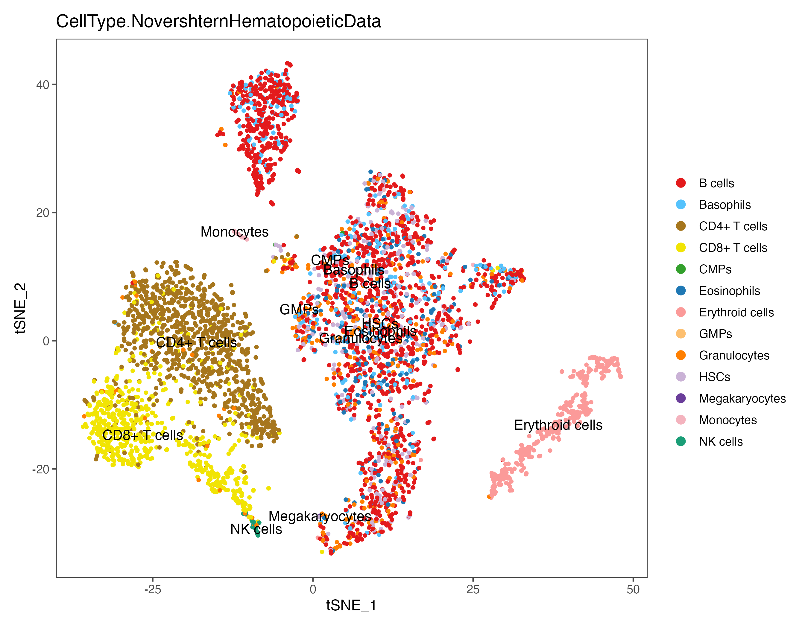
# tsne
p <- DimPlot(sce, reduction = "tsne", pt.size = 1, label = TRUE, label.size = 4,
group.by = "CellType.BlueprintEncodeData", cols = color.lib) + theme_few()
ggsave(paste0(out.path, "/8.SingleR.tsne.BlueprintEncodeData.pdf"), p, width = 9, height = 7)
p <- DimPlot(sce, reduction = "tsne", pt.size = 1, label = TRUE, label.size = 4,
group.by = "CellType.HumanPrimaryCellAtlasData", cols = color.lib) + theme_few()
ggsave(paste0(out.path, "/8.SingleR.tsne.HumanPrimaryCellAtlasData.pdf"), p, width = 9, height = 7)
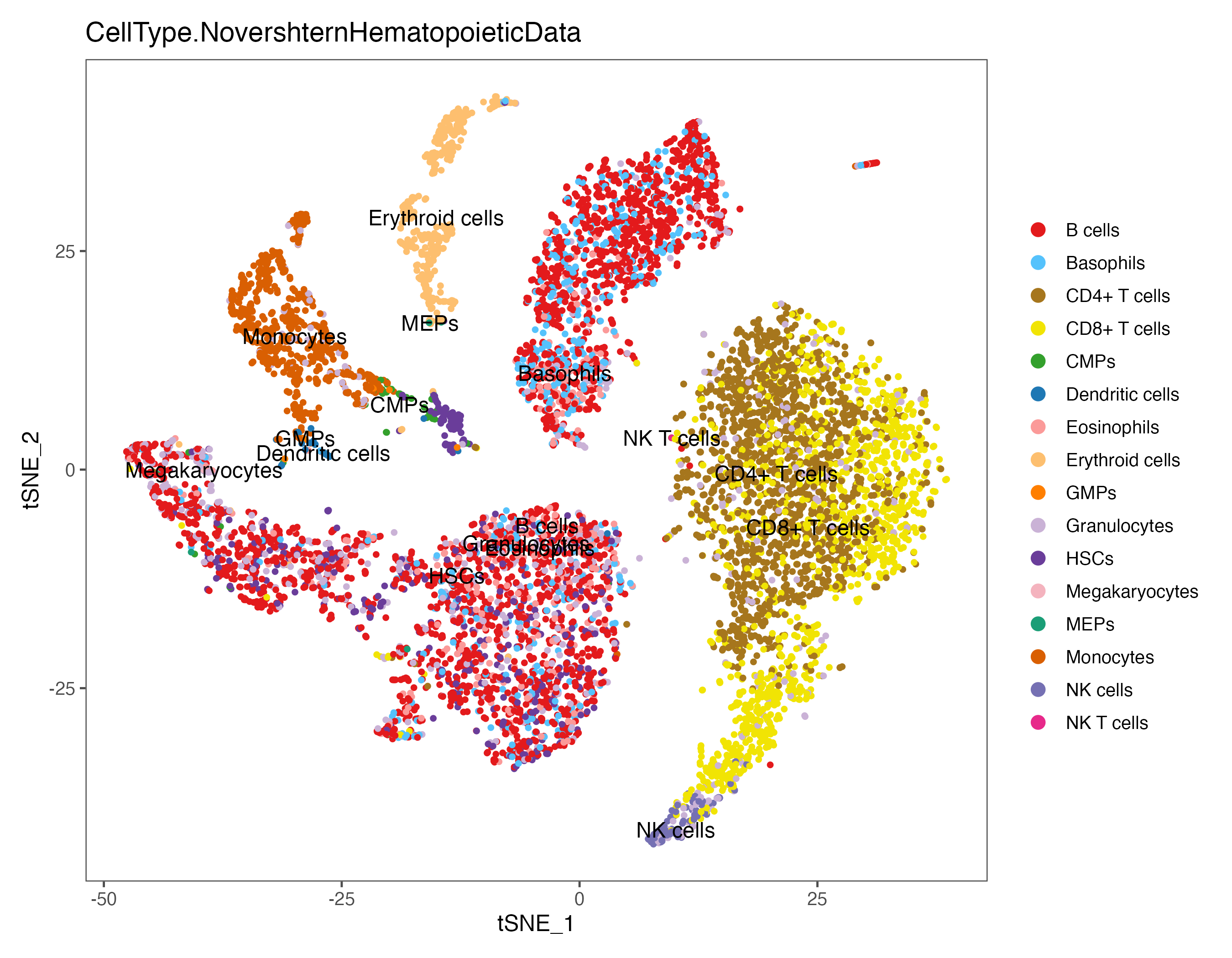
p <- DimPlot(sce, reduction = "tsne", pt.size = 1, label = TRUE, label.size = 4,
group.by = "CellType.NovershternHematopoieticData", cols = color.lib) + theme_few()
ggsave(paste0(out.path, "/8.SingleR.tsne.NovershternHematopoieticData.pdf"), p, width = 9, height = 7)
#----------------------------------------------------------------------------------
# Step 11: Finding differentially expressed features (find marker)
#----------------------------------------------------------------------------------
ident.meta <- data.frame(table(sce@meta.data$seurat_clusters))
colnames(ident.meta) <- c("Cluster","CellCount")
write.xlsx(ident.meta, paste0(out.path, "/9.CellCount.xlsx"), overwrite = T)
# Cluster CellCount
# 0 941
# 1 604
# 2 562
# 3 539
# 4 280
# 5 208
# find marker
sce <- BuildClusterTree(object = sce)
all.markers <- FindAllMarkers(object = sce, only.pos = TRUE, logfc.threshold = 0.1, min.pct = 0.1)
all.markers <- all.markers[which(all.markers$p_val_adj < 0.05 & all.markers$avg_log2FC > 0), ]
write.xlsx(all.markers, paste0(out.path, "/10.top.markers.xlsx"), overwrite = T)
# plot top 10 markers
all.markers <- read.xlsx(paste0(out.path, "/10.top.markers.xlsx"))
all.markers <- all.markers[which(all.markers$pct.1 > 0.25), ]
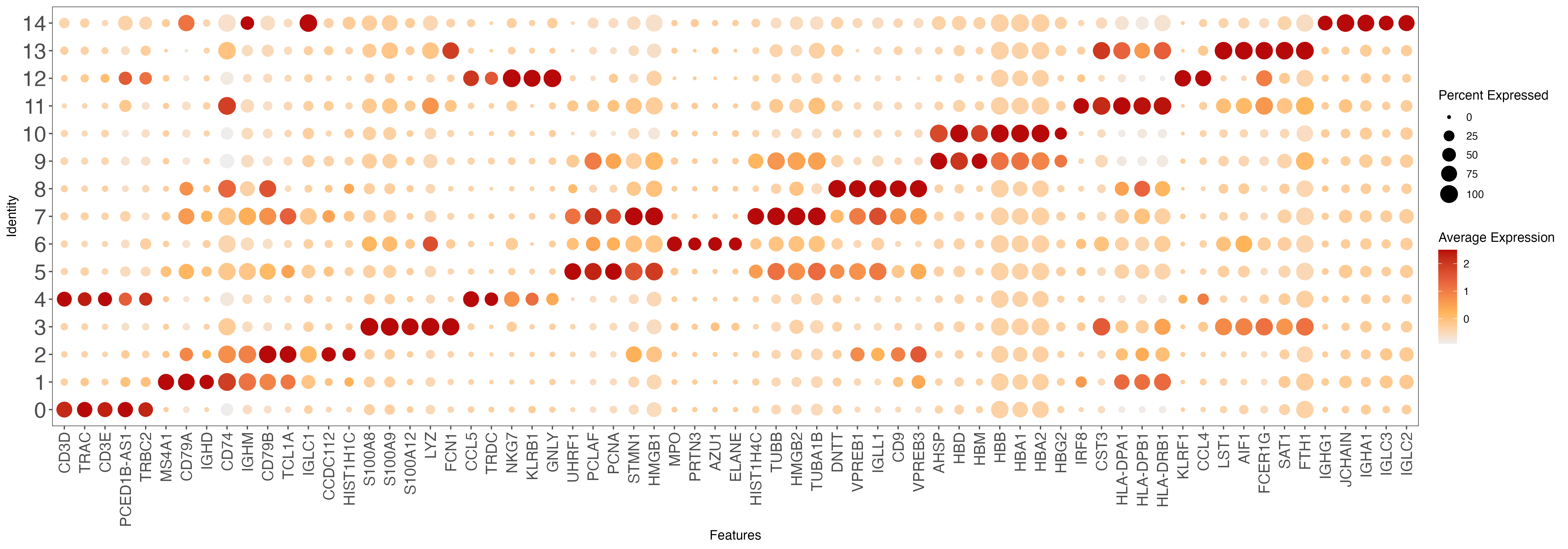
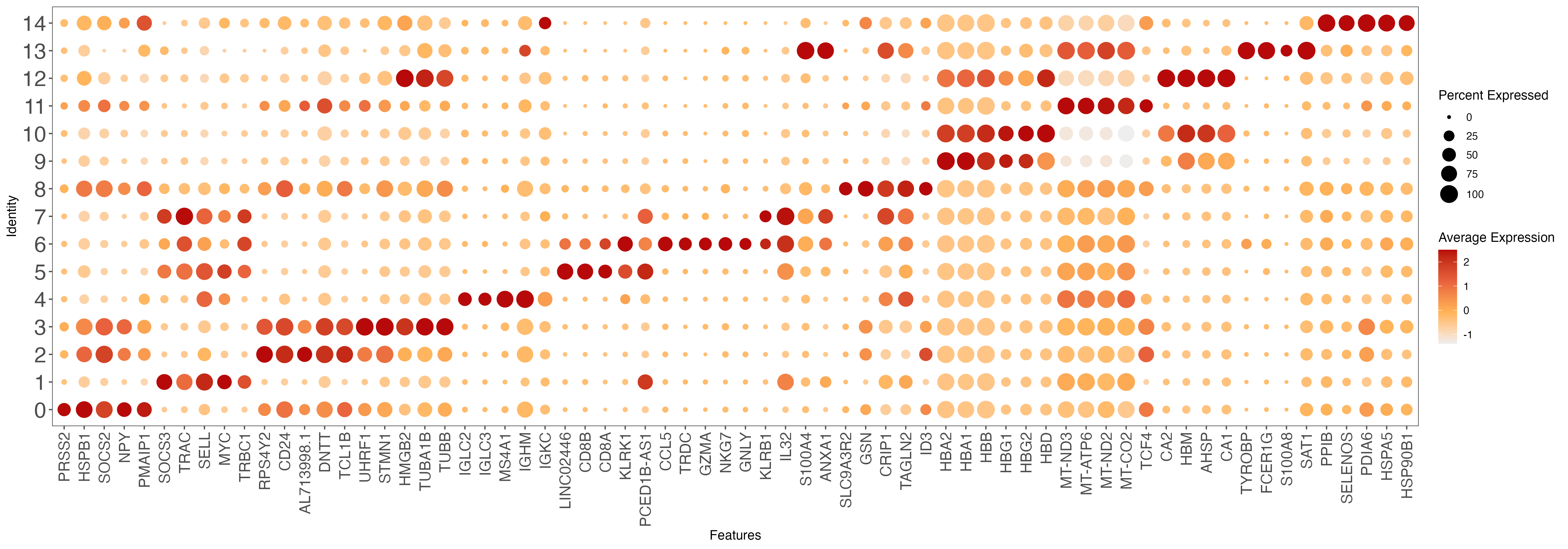
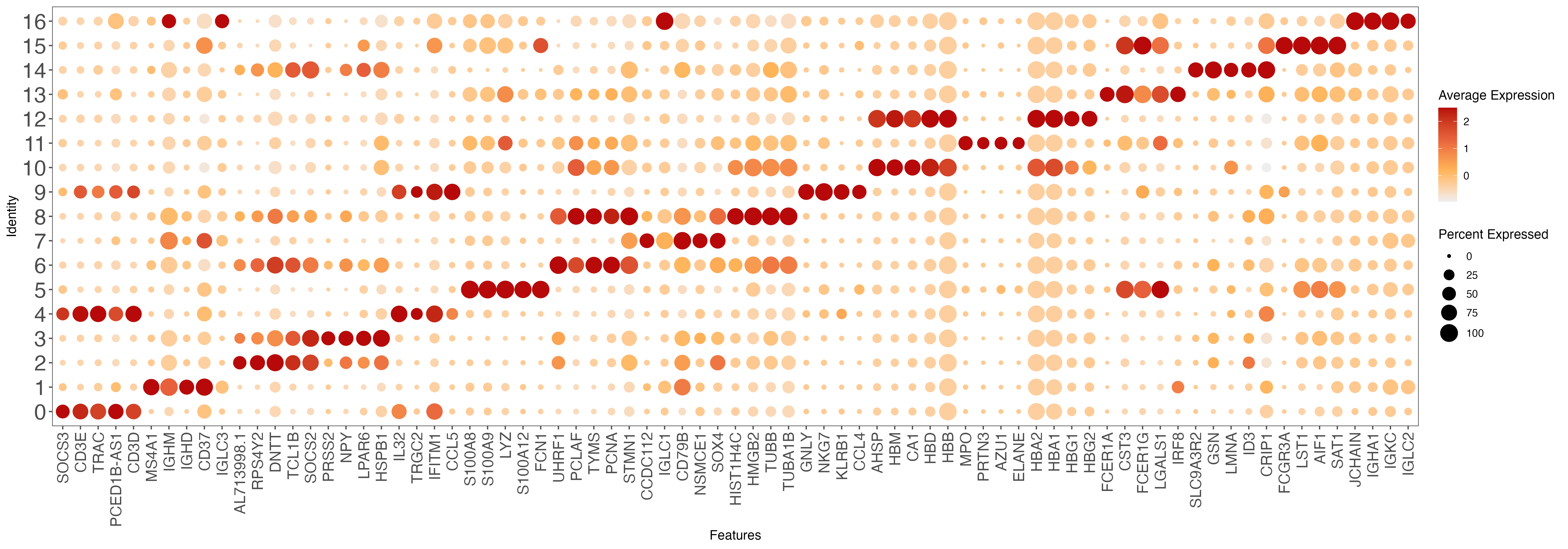
top10 <- all.markers %>% group_by(cluster) %>% top_n(n = 5, wt = avg_log2FC)
gene.list <- unique(top10$gene)
p <- DotPlot(sce, features = gene.list, dot.scale = 8, cols = c("#DDDDDD", "#003366" ), col.min = -2) + RotatedAxis()
p <- p + theme_few() + theme(axis.text.x = element_text(angle = 90, hjust = 1, vjust = 0.5, size = 14))
p <- p + theme(axis.text.y = element_text(size = 20))
p <- p + scale_size(range = c(1, 7))
p <- p + gradient_color(c("#EEEEEE","#ffb459","#e8613c","#b70909"))
ggsave(paste0(out.path, "/10.top.markers.pdf"), p, width = 20, height = 7) ## marker genes dot plot
#----------------------------------------------------------------------------------
# Step 12: check wellknown markers
#----------------------------------------------------------------------------------
# Expression for each cluster
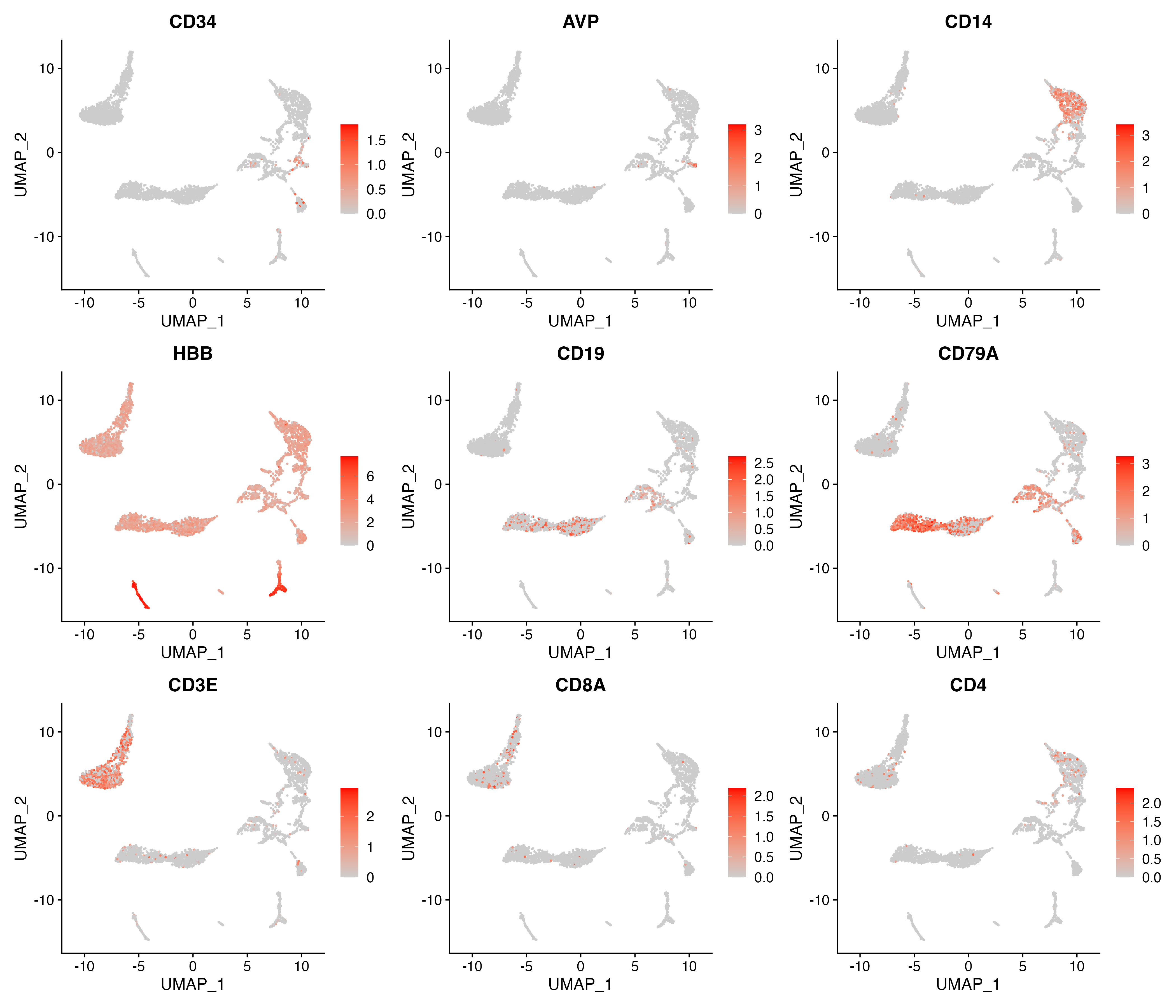
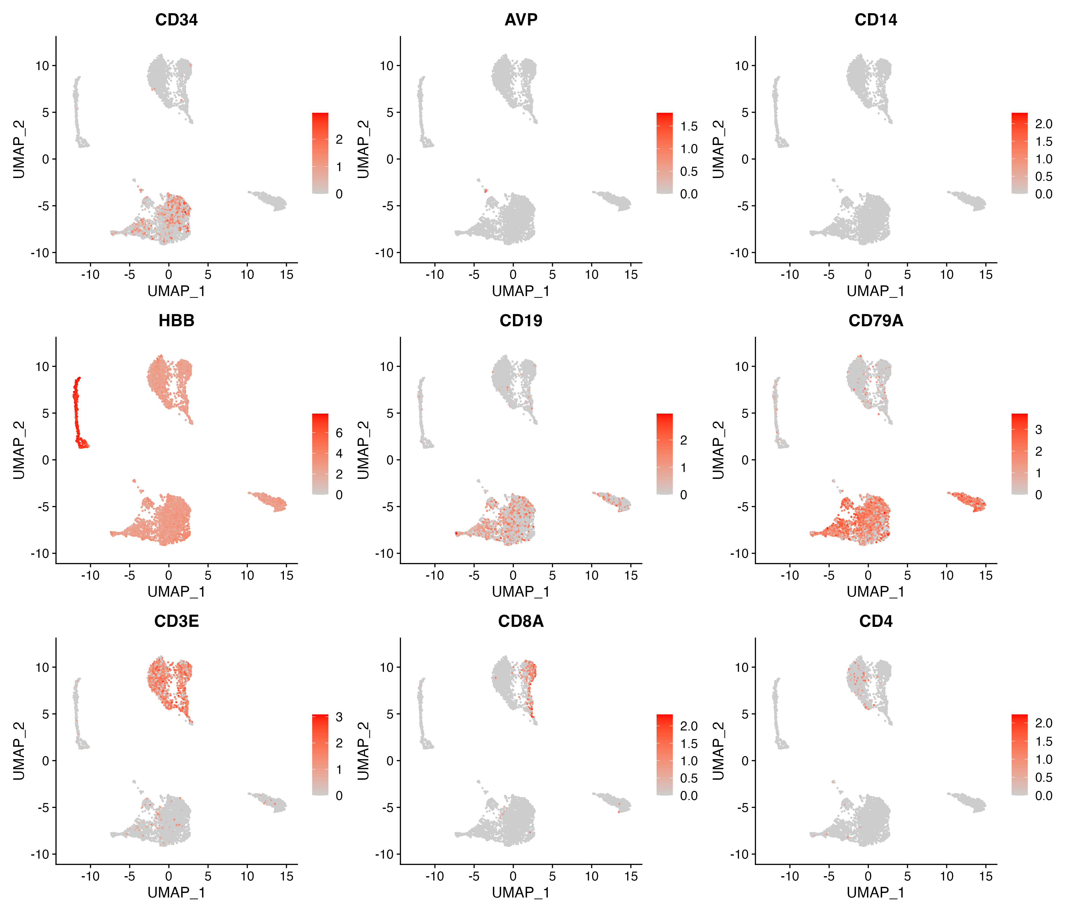
p <- FeaturePlot(object = sce, features = c("CD34","AVP","CD14","HBB","CD19","CD79A","CD3E","CD8A","CD4"),
cols = c("#CCCCCC", "red"), pt.size = 0.3, ncol = 3,
reduction = "umap")
ggsave(paste0(out.path, "/11.featurePlot.pdf"), p, width = 14, height = 12)
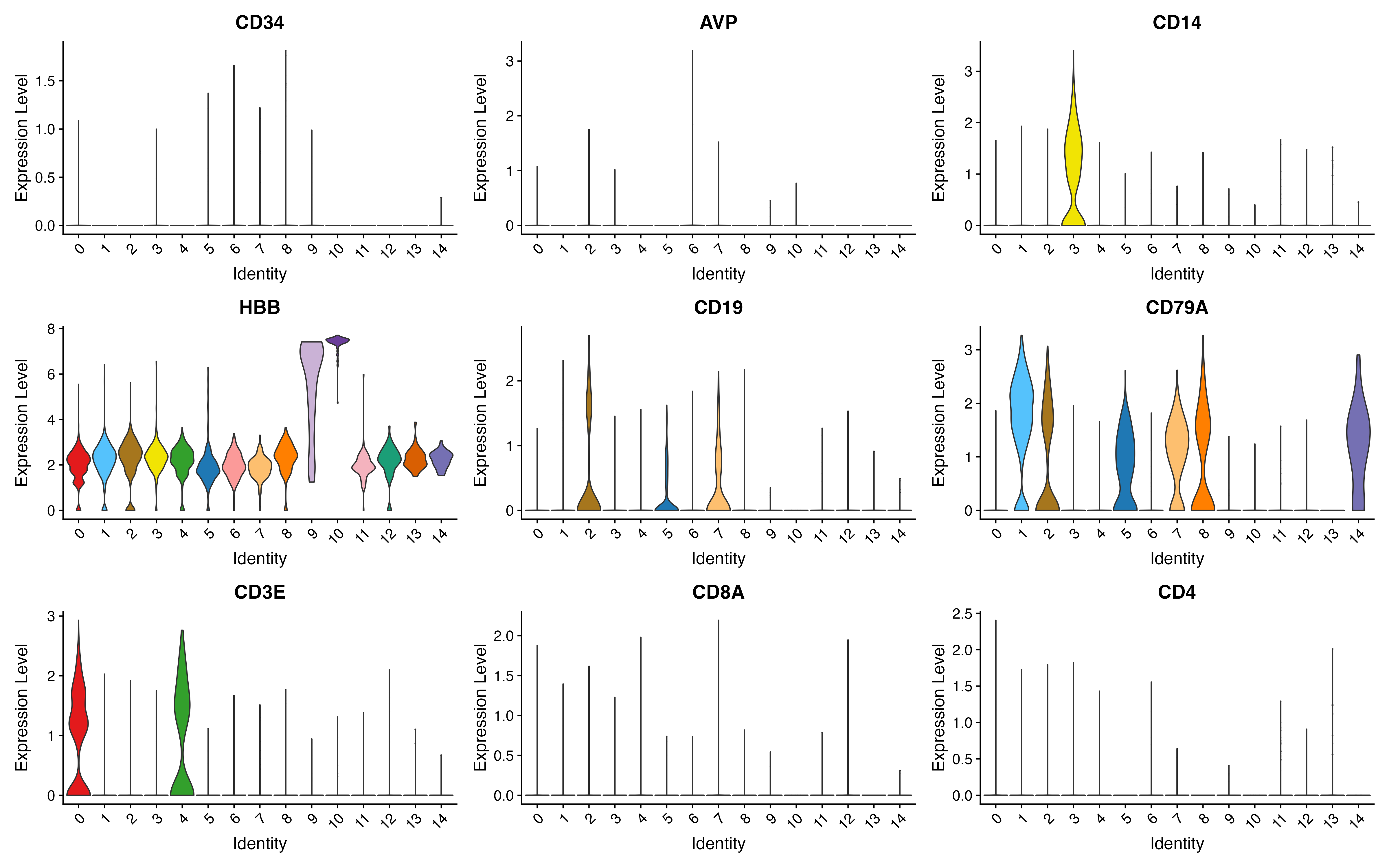
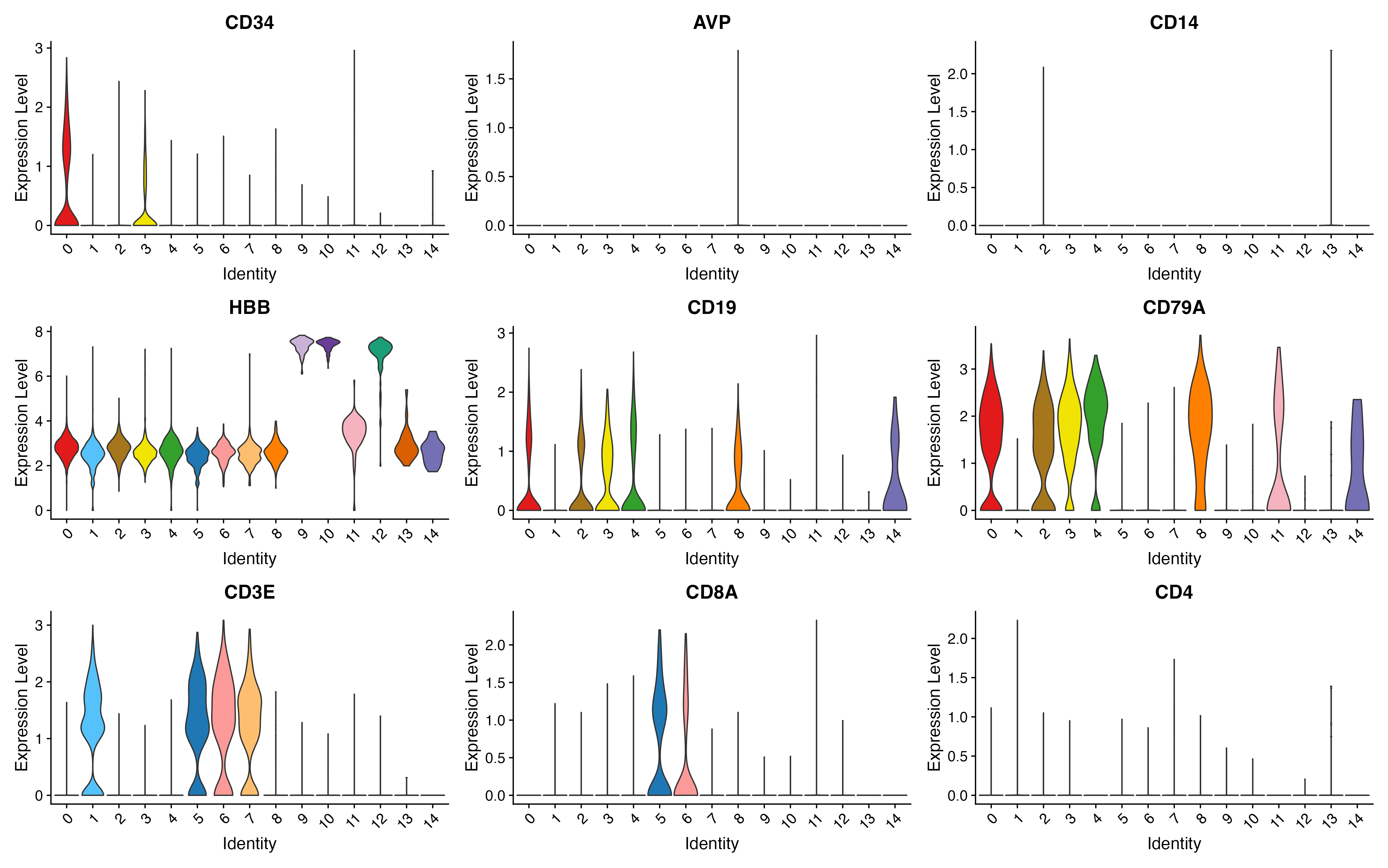
p <- VlnPlot(object = sce, features = c("CD34","AVP","CD14","HBB","CD19","CD79A","CD3E","CD8A","CD4"),
             pt.size = 0, cols = color.lib, slot = "data", ncol = 3)
ggsave(paste0(out.path, "/11.VlnPlot.pdf"), p, width = 16, height = 10)
## save object
dir.create("./output/obj",recursive = T)
saveRDS(sce, paste0("./output/obj/20231011.", sample.name, ".rds"))
BALL_BM
library(Seurat)
library(dplyr)
library(Matrix)
library(gplots)
library(matrixStats)
library(ggpubr)
library(openxlsx)
library(stringr)
library(ggthemes)
library(pheatmap)
library(SingleR)
library(monocle3) # devtools::install_github('cole-trapnell-lab/monocle3')
library(harmony)  # install.packages("harmony")
#----------------------------------------------------------------------------------
#  Step 1: setting
#----------------------------------------------------------------------------------
rm(list = ls())
color.lib <- c("#E31A1C", "#55c2fc", "#A6761D", "#F1E404", "#33A02C", "#1F78B4",
               "#FB9A99", "#FDBF6F", "#FF7F00", "#CAB2D6", "#6A3D9A", "#F4B3BE",
               "#1B9E77", "#D95F02", "#7570B3", "#E7298A", "#66A61E", "#E6AB02",
               "#F4A11D", "#8DC8ED", "#4C6CB0", "#8A1C1B", "#CBCC2B", "#EA644C",
               "#634795", "#005B1D", "#26418A", "#CB8A93", "#B2DF8A", "#E22826",
               "#A6CEE3", "#F4D31D", "#F4A11D", "#82C800", "#8B5900", "#858ED1",
               "#FF72E1", "#CB50B2", "#007D9B", "#26418A", "#8B495F", "#FF394B")

sample.name = "BALL_BM"
message(sample.name)
# Set output path
out.path <- paste0("output/", sample.name) #system(sprintf("mkdir %s", out.path))
dir.create(out.path,recursive = T)
#----------------------------------------------------------------------------------
#  Step 2: Setup the Seurat Object
#----------------------------------------------------------------------------------
# load data from data folder
scell.data <- Read10X(data.dir = paste0("data/", sample.name) )
colnames(scell.data) <- str_replace_all(colnames(scell.data), "1", sample.name)
# Initialize the Seurat object with the raw (non-normalized data)
sce <- CreateSeuratObject(counts = scell.data, project = "sce", min.cells = 0, min.features = 0)
# Add sample information
sce@meta.data$Sample = sample.name
sce
head(sce@meta.data)
#----------------------------------------------------------------------------------
#  Step 3: QC and selecting cells
#----------------------------------------------------------------------------------
# key challenges: ensure that only single, live cells are included in downstream analysis
## mitochondrial gene
sce[["percent.mt"]] <- PercentageFeatureSet(sce, pattern = "^MT-")
sce
summary(sce@meta.data$percent.mt)
# Visualize QC metrics as a violin plot
pdf(paste0(out.path, "/1.vlnplot.pdf"), width = 12, height = 7)
VlnPlot(sce, features = c("nFeature_RNA", "nCount_RNA", "percent.mt"), group.by = "orig.ident", ncol = 3)
dev.off()
# visualize feature-feature relationships
pdf(paste0(out.path, "/1.geneplot.pdf"), width = 12, height = 7)
plot1 <- FeatureScatter(sce, feature1 = "nCount_RNA", feature2 = "percent.mt")
plot2 <- FeatureScatter(sce, feature1 = "nCount_RNA", feature2 = "nFeature_RNA")
plot1 + plot2
dev.off()
## QC : selecting cells
sce <- subset(sce, subset = nFeature_RNA > 200 & percent.mt < 20)
sce
# plot after QC
pdf(paste0(out.path, "/2.filter.vlnplot.pdf"), width = 12, height = 7)
VlnPlot(sce, features = c("nFeature_RNA", "nCount_RNA", "percent.mt"),  group.by = "orig.ident", ncol = 3)
dev.off()
pdf(paste0(out.path, "/2.filter.geneplot.pdf"), width = 12, height = 7)
plot1 <- FeatureScatter(sce, feature1 = "nCount_RNA", feature2 = "percent.mt")
plot2 <- FeatureScatter(sce, feature1 = "nCount_RNA", feature2 = "nFeature_RNA")
plot1 + plot2
dev.off()
#----------------------------------------------------------------------------------
# Step 4: Normalizing the data
#----------------------------------------------------------------------------------
# After removing unwanted cells from the dataset, the next step is to normalize the data.
sce <- NormalizeData(sce, normalization.method = "LogNormalize", scale.factor = ncol(sce))
# By default, we employ a global-scaling normalization method “LogNormalize” that normalizes the feature expression measurements for each cell by the total expression, multiplies this by a scale factor (10,000 by default), and log-transforms the result. Normalized values are stored in pbmc[["RNA"]]@data
sce[["RNA"]]@data[1:20,1:5]
#----------------------------------------------------------------------------------
# Step 5: Identification of highly variable features (feature selection)
#----------------------------------------------------------------------------------
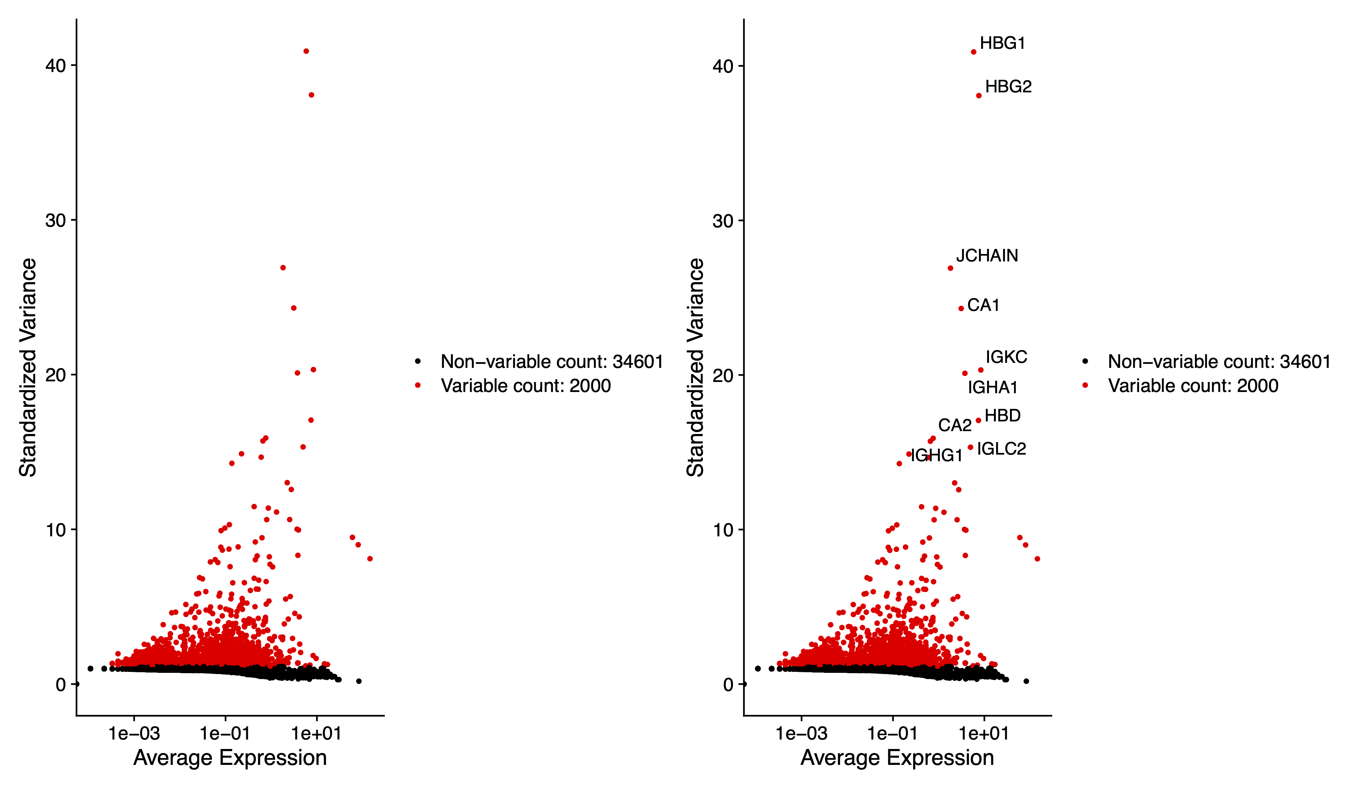
# We next calculate a subset of features that exhibit high cell-to-cell variation in the dataset
sce <- FindVariableFeatures(sce, selection.method = "vst", nfeatures = 2000)
# Identify the 10 most highly variable genes
top10 <- head(VariableFeatures(sce), 10)
# plot variable features with and without labels
pdf(paste0(out.path, "/3.VariableFeaturePlot.pdf"), width = 12, height = 7)
plot1 <- VariableFeaturePlot(sce)
plot2 <- LabelPoints(plot = plot1, points = top10, repel = TRUE)
plot1 + plot2
dev.off()
#----------------------------------------------------------------------------------
#  Step 6: Scaling the data
#----------------------------------------------------------------------------------
# linear transformation: pre-processing step prior to dimensional reduction techniques like PCA
all.genes <- rownames(sce)
sce <- ScaleData(sce, features = VariableFeatures(sce))
sce <- RunPCA(sce, features = VariableFeatures(object = sce))
p <- DimPlot(sce, reduction = "pca") + theme_few()
ggsave(paste0(out.path, "/4.PCA.pdf"), p, width = 8.5, height = 7)
#----------------------------------------------------------------------------------
#  Step 7: Cluster the cells
#----------------------------------------------------------------------------------
sce <- FindNeighbors(sce, reduction = "pca", dims = 1:20)
sce <- FindClusters(sce, resolution = 0.8)
#----------------------------------------------------------------------------------
#  Step 8: Run non-linear dimensional reduction (UMAP/tSNE)
#----------------------------------------------------------------------------------
# to learn the underlying manifold of the data in order to place similar cells together in low-dimensional space
# If you haven't installed UMAP, you can do so via reticulate::py_install(packages =
# 'umap-learn')
sce <- RunTSNE(sce, reduction = "pca", dims = 1:20, perplexity = 30)
sce <- RunUMAP(sce, reduction = "pca", dims = 1:20)
# plot
# umap
p <- DimPlot(sce, reduction = "umap", pt.size = 1,
             cols = color.lib) + theme_few()
ggsave(paste0(out.path, "/5.UMAP.cluster.pdf"), p, width = 8.5, height = 7)

p <- DimPlot(sce, reduction = "umap", pt.size = 1, label = TRUE, label.size = 10,
             cols = color.lib) + theme_few()
ggsave(paste0(out.path, "/5.UMAP.cluster.label.pdf"), p, width = 8.5, height = 7)
# tsne
p <- DimPlot(sce, reduction = "tsne", pt.size = 1,
             cols = color.lib) + theme_few()
ggsave(paste0(out.path, "/6.tSNE.cluster.pdf"), p, width = 8.5, height = 7)

p <- DimPlot(sce, reduction = "tsne", pt.size = 1, label = TRUE, label.size = 10,
             cols = color.lib) + theme_few()
ggsave(paste0(out.path, "/6.tSNE.cluster.label.pdf"), p, width = 8.5, height = 7)
#----------------------------------------------------------------------------------
#  Step 9: Cell cycle
#----------------------------------------------------------------------------------
# build-in cell cycle genes
cc.genes
sce <- CellCycleScoring(sce, s.features = cc.genes$s.genes, g2m.features = cc.genes$g2m.genes)

p <- DimPlot(sce, reduction = "umap", pt.size = 1, label = FALSE,
             group.by = "Phase", cols = color.lib) + theme_few()
ggsave(paste0(out.path, "/7.CC.phase.pdf"), p, width = 8.5, height = 7)

p <- VlnPlot(sce, features = "S.Score", pt.size = 0,
             group.by = "seurat_clusters", cols = color.lib) + theme_few()
ggsave(paste0(out.path, "/7.CC.score.S.Score.pdf"), p, width = 10, height = 5)

p <- VlnPlot(sce, features = "G2M.Score", pt.size = 0,
             group.by = "seurat_clusters", cols = color.lib) + theme_few()
ggsave(paste0(out.path, "/7.CC.score.G2M.Score.pdf"), p, width = 10, height = 5)
#----------------------------------------------------------------------------------
#  Step 10: SingleR annotation
#----------------------------------------------------------------------------------
# first, load reference datasets. Then, annotate your query data based on reference datasets.
ref <- readRDS(file = "./data/SingleR/hs.BlueprintEncodeData.RDS")
pred.BlueprintEncodeData <- SingleR(test = sce@assays$RNA@data, ref = ref, labels = ref$label.main)

ref <- readRDS(file = "./data/SingleR/hs.HumanPrimaryCellAtlasData.RDS")
pred.HumanPrimaryCellAtlasData <- SingleR(test = sce@assays$RNA@data, ref = ref, labels = ref$label.main)

ref <- readRDS(file = "./data/SingleR/NovershternHematopoieticData.RDS")
pred.NovershternHematopoieticData <- SingleR(test = sce@assays$RNA@data, ref = ref, labels = ref$label.main)
# add annotations to meta data
sce@meta.data$CellType.BlueprintEncodeData <- pred.BlueprintEncodeData$labels
sce@meta.data$CellType.HumanPrimaryCellAtlasData <- pred.HumanPrimaryCellAtlasData$labels
sce@meta.data$CellType.NovershternHematopoieticData <- pred.NovershternHematopoieticData$labels
# plot with annotations
# umap
p <- DimPlot(sce, reduction = "umap", pt.size = 1, label = TRUE, label.size = 4,
             group.by = "CellType.BlueprintEncodeData", cols = color.lib) + theme_few()
ggsave(paste0(out.path, "/8.SingleR.umap.BlueprintEncodeData.pdf"), p, width = 9, height = 7)

p <- DimPlot(sce, reduction = "umap", pt.size = 1, label = TRUE, label.size = 4,
             group.by = "CellType.HumanPrimaryCellAtlasData", cols = color.lib) + theme_few()
ggsave(paste0(out.path, "/8.SingleR.umap.HumanPrimaryCellAtlasData.pdf"), p, width = 9, height = 7)

p <- DimPlot(sce, reduction = "umap", pt.size = 1, label = TRUE, label.size = 4,
             group.by = "CellType.NovershternHematopoieticData", cols = color.lib) + theme_few()
ggsave(paste0(out.path, "/8.SingleR.umap.NovershternHematopoieticData.pdf"), p, width = 9, height = 7)
# tsne
p <- DimPlot(sce, reduction = "tsne", pt.size = 1, label = TRUE, label.size = 4,
             group.by = "CellType.BlueprintEncodeData", cols = color.lib) + theme_few()
ggsave(paste0(out.path, "/8.SingleR.tsne.BlueprintEncodeData.pdf"), p, width = 9, height = 7)

p <- DimPlot(sce, reduction = "tsne", pt.size = 1, label = TRUE, label.size = 4,
             group.by = "CellType.HumanPrimaryCellAtlasData", cols = color.lib) + theme_few()
ggsave(paste0(out.path, "/8.SingleR.tsne.HumanPrimaryCellAtlasData.pdf"), p, width = 9, height = 7)

p <- DimPlot(sce, reduction = "tsne", pt.size = 1, label = TRUE, label.size = 4,
             group.by = "CellType.NovershternHematopoieticData", cols = color.lib) + theme_few()
ggsave(paste0(out.path, "/8.SingleR.tsne.NovershternHematopoieticData.pdf"), p, width = 9, height = 7)
#----------------------------------------------------------------------------------
#  Step 11: Finding differentially expressed features (find marker)
#----------------------------------------------------------------------------------
ident.meta <- data.frame(table(sce@meta.data$seurat_clusters))
colnames(ident.meta) <- c("Cluster","CellCount")
write.xlsx(ident.meta, paste0(out.path, "/9.CellCount.xlsx"), overwrite = T)
#   Cluster CellCount
# 1       0       920
# 2       1       875
# 3       2       526
# 4       3       481
# 5       4       472
# 6       5       417

# find marker
sce <- BuildClusterTree(object = sce)
all.markers <- FindAllMarkers(object = sce, only.pos = TRUE, logfc.threshold = 0.1, min.pct = 0.1)
all.markers <- all.markers[which(all.markers$p_val_adj < 0.05 & all.markers$avg_log2FC > 0), ]
write.xlsx(all.markers, paste0(out.path, "/10.top.markers.xlsx"), overwrite = T)
# plot top 10 markers
all.markers <- read.xlsx(paste0(out.path, "/10.top.markers.xlsx"))
all.markers <- all.markers[which(all.markers$pct.1 > 0.25), ]
top10 <- all.markers %>% group_by(cluster) %>% top_n(n = 5, wt = avg_log2FC)
gene.list <- unique(top10$gene)
p <- DotPlot(sce, features = gene.list, dot.scale = 8, cols = c("#DDDDDD", "#003366" ), col.min = -2) + RotatedAxis()
p <- p + theme_few() + theme(axis.text.x = element_text(angle = 90, hjust = 1, vjust = 0.5, size = 14))
p <- p + theme(axis.text.y = element_text(size = 20))
p <- p + scale_size(range = c(1, 7))
p <- p + gradient_color(c("#EEEEEE","#ffb459","#e8613c","#b70909"))
ggsave(paste0(out.path, "/10.top.markers.pdf"), p, width = 20, height = 7) ## marker genes dot plot
#----------------------------------------------------------------------------------
#  Step 12: check wellknown markers
#----------------------------------------------------------------------------------
# Expression for each cluster
p <- FeaturePlot(object = sce, features = c("CD34","AVP","CD14","HBB","CD19","CD79A","CD3E","CD8A","CD4"),
                 cols = c("#CCCCCC", "red"), pt.size = 0.3, ncol = 3,
                 reduction = "umap")
ggsave(paste0(out.path, "/11.featurePlot.pdf"), p, width = 14, height = 12)
p <- VlnPlot(object = sce, features = c("CD34","AVP","CD14","HBB","CD19","CD79A","CD3E","CD8A","CD4"),
             pt.size = 0, cols = color.lib, slot = "data", ncol = 3)
ggsave(paste0(out.path, "/11.VlnPlot.pdf"), p, width = 16, height = 10)
## save object
dir.create("./output/obj",recursive = T)
saveRDS(sce, paste0("./output/obj/20231011.", sample.name, ".rds"))
Integration
library(Seurat)
library(dplyr)
library(Matrix)
library(gplots)
library(matrixStats)
library(ggpubr)
library(openxlsx)
library(stringr)
library(ggthemes)
library(pheatmap)
library(harmony)
library(SingleR)
#----------------------------------------------------------------------------------
# Step 1: setting
#----------------------------------------------------------------------------------
rm(list = ls())
color.lib <- c("#E31A1C", "#55c2fc", "#A6761D", "#F1E404", "#33A02C", "#1F78B4",
"#FB9A99", "#FDBF6F", "#FF7F00", "#CAB2D6", "#6A3D9A", "#F4B3BE",
"#1B9E77", "#D95F02", "#7570B3", "#E7298A", "#66A61E", "#E6AB02",
"#F4A11D", "#8DC8ED", "#4C6CB0", "#8A1C1B", "#CBCC2B", "#EA644C",
"#634795", "#005B1D", "#26418A", "#CB8A93", "#B2DF8A", "#E22826",
"#A6CEE3", "#F4D31D", "#F4A11D", "#82C800", "#8B5900", "#858ED1",
"#FF72E1", "#CB50B2", "#007D9B", "#26418A", "#8B495F", "#FF394B")
sample.list <- c("BALL_BM","CTRL_BM")
out.path <- "output/merge_BALL_CTRL"
dir.create(out.path) # system(sprintf("mkdir %s", out.path))
#----------------------------------------------------------------------------------
# Step 2: merge expression profile
#----------------------------------------------------------------------------------
exp.data <- NULL
meta.data <- NULL
for (kkk in 1:length(sample.list)) {
message(kkk, " ", sample.list[kkk])
obj.raw <- readRDS(paste0("./output/obj/20231011.", sample.list[kkk], ".rds"))
exp.data <- cbind(exp.data, obj.raw@assays$RNA@counts )
meta.data <- rbind(meta.data, obj.raw@meta.data[, c("Sample","CellType.BlueprintEncodeData","CellType.HumanPrimaryCellAtlasData","CellType.NovershternHematopoieticData")] )
}
#----------------------------------------------------------------------------------
# Step 3: Setup the Seurat Object
#----------------------------------------------------------------------------------
sce <- CreateSeuratObject(counts = exp.data, project = "sce", min.cells = 0, min.features = 0)
sce[["percent.mt"]] <- PercentageFeatureSet(sce, pattern = "^MT-")
sce
summary(sce@meta.data$percent.mt)
sce@meta.data <- cbind(sce@meta.data, meta.data)
#----------------------------------------------------------------------------------
# Step 4: QC
#----------------------------------------------------------------------------------
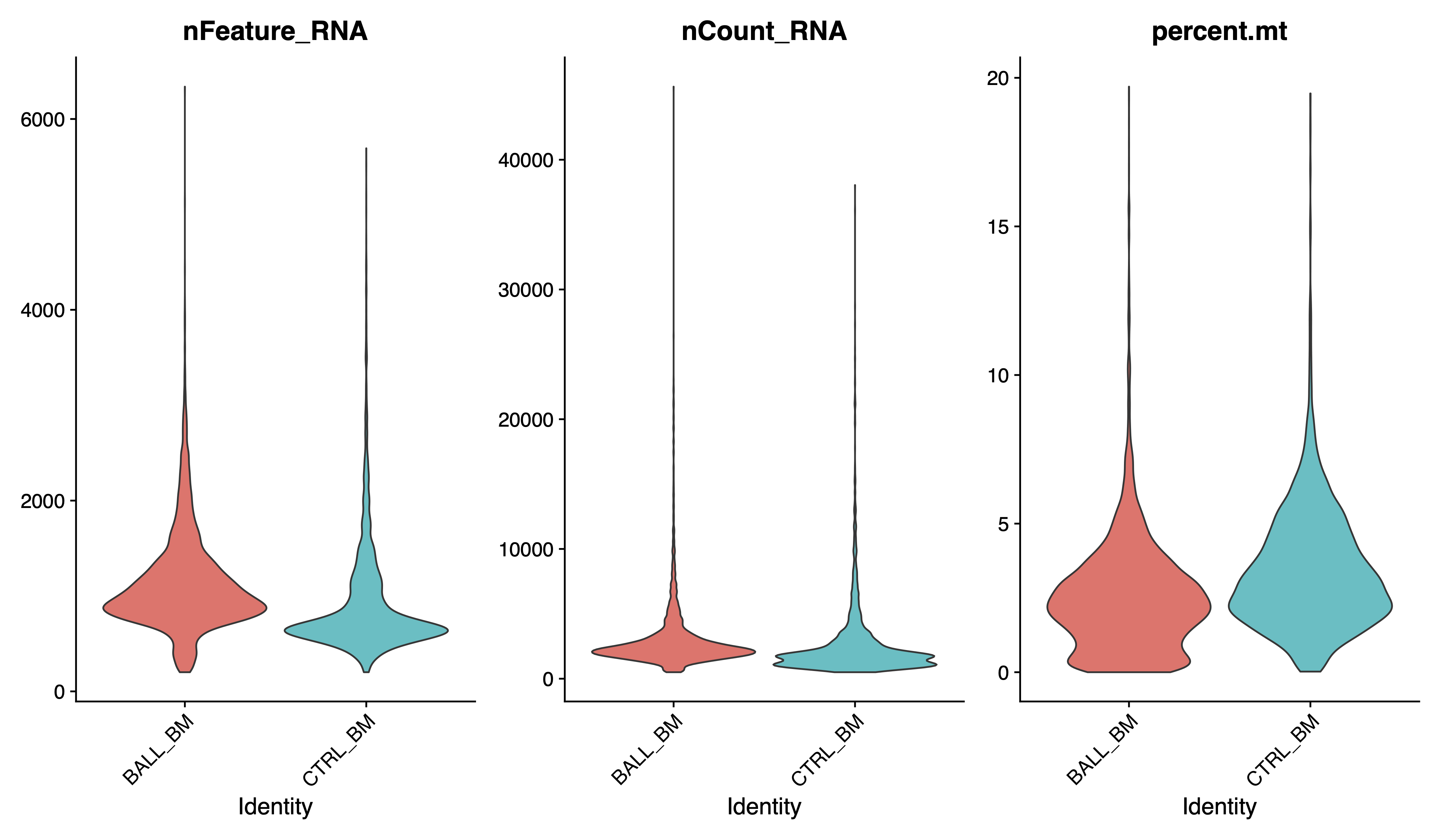
pdf(paste0(out.path, "/1.raw.vlnplot.pdf"), width = 12, height = 7)
VlnPlot(sce, features = c("nFeature_RNA", "nCount_RNA", "percent.mt"), pt.size = 0, group.by = "Sample", ncol = 3)
dev.off()

pdf(paste0(out.path, "/1.raw.geneplot.pdf"), width = 12, height = 7)
plot1 <- FeatureScatter(sce, feature1 = "nCount_RNA", feature2 = "percent.mt")
plot2 <- FeatureScatter(sce, feature1 = "nCount_RNA", feature2 = "nFeature_RNA")
plot1 + plot2
dev.off()
## QC : selecting cells
sce <- subset(sce, subset = nFeature_RNA > 500 & percent.mt < 10 & nCount_RNA < 50000)
# plot after QC
pdf(paste0(out.path, "/2.filter.vlnplot.pdf"), width = 12, height = 7)
VlnPlot(sce, features = c("nFeature_RNA", "nCount_RNA", "percent.mt"), pt.size = 0, group.by = "Sample", ncol = 3)
dev.off()
pdf(paste0(out.path, "/2.filter.geneplot.pdf"), width = 12, height = 7)
plot1 <- FeatureScatter(sce, feature1 = "nCount_RNA", feature2 = "percent.mt")
plot2 <- FeatureScatter(sce, feature1 = "nCount_RNA", feature2 = "nFeature_RNA")
plot1 + plot2
dev.off()

#----------------------------------------------------------------------------------
#  Step 5: Normalizing the data
#----------------------------------------------------------------------------------
sce <- NormalizeData(sce, normalization.method = "LogNormalize", scale.factor = ncol(sce) )
sce <- FindVariableFeatures(sce, selection.method = "vst", nfeatures = 2000)
#----------------------------------------------------------------------------------
#  Step 6: Identification of highly variable features (feature selection)
#----------------------------------------------------------------------------------
# Identify the 10 most highly variable genes
top10 <- head(VariableFeatures(sce), 10)
# plot variable features with and without labels
pdf(paste0(out.path, "/3.VariableFeaturePlot.pdf"), width = 12, height = 7)
plot1 <- VariableFeaturePlot(sce)
plot2 <- LabelPoints(plot = plot1, points = top10, repel = TRUE)
plot1 + plot2
dev.off()
#----------------------------------------------------------------------------------
# Step 7: Scaling the data
#----------------------------------------------------------------------------------
all.genes <- rownames(sce)
sce <- ScaleData(sce, features = VariableFeatures(sce))
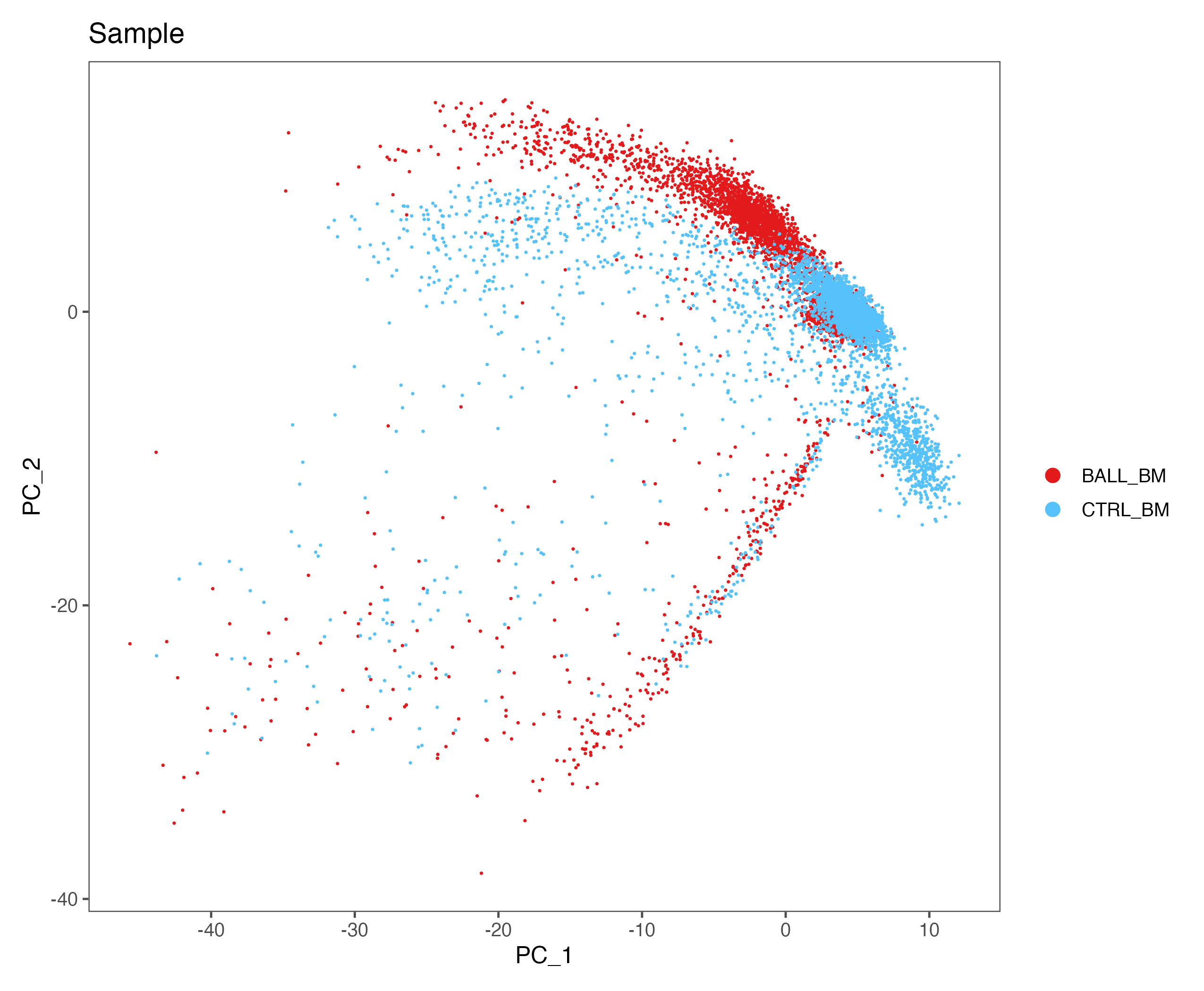
sce <- RunPCA(sce, features = VariableFeatures(object = sce))
p <- DimPlot(sce, reduction = "pca", group.by = "Sample", cols = color.lib) + theme_few()
ggsave(paste0(out.path, "/4.PCA.pdf"), p, width = 8.5, height = 7)
#----------------------------------------------------------------------------------
# Step 8: Harmony 批次矫正
#----------------------------------------------------------------------------------
length(VariableFeatures(sce))
sce <- RunHarmony(sce, "Sample")
#----------------------------------------------------------------------------------
# Step 9: Cluster the cells
#----------------------------------------------------------------------------------
sce <- FindNeighbors(sce, reduction = "harmony", dims = 1:20)
sce <- FindClusters(sce, resolution = 0.8)
#----------------------------------------------------------------------------------
# Step 10: Run non-linear dimensional reduction (UMAP/tSNE)
#----------------------------------------------------------------------------------
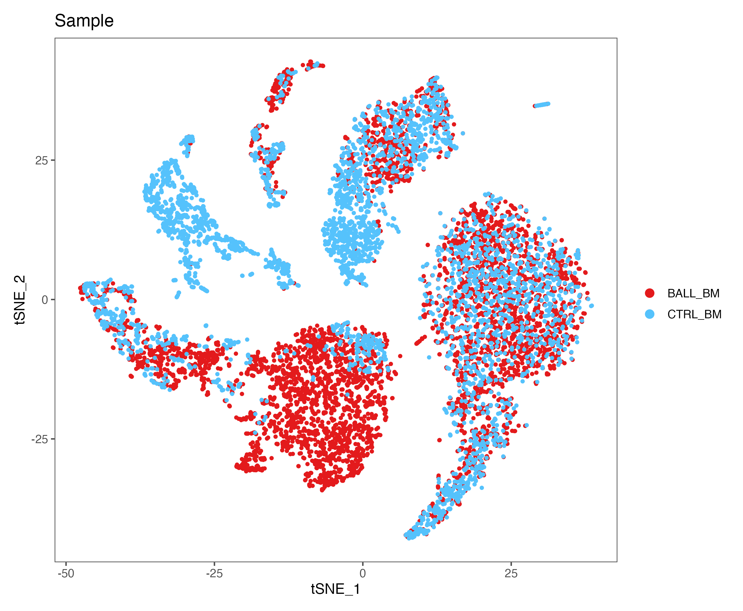
sce <- RunTSNE(sce, reduction = "harmony", dims = 1:20, perplexity = 30)
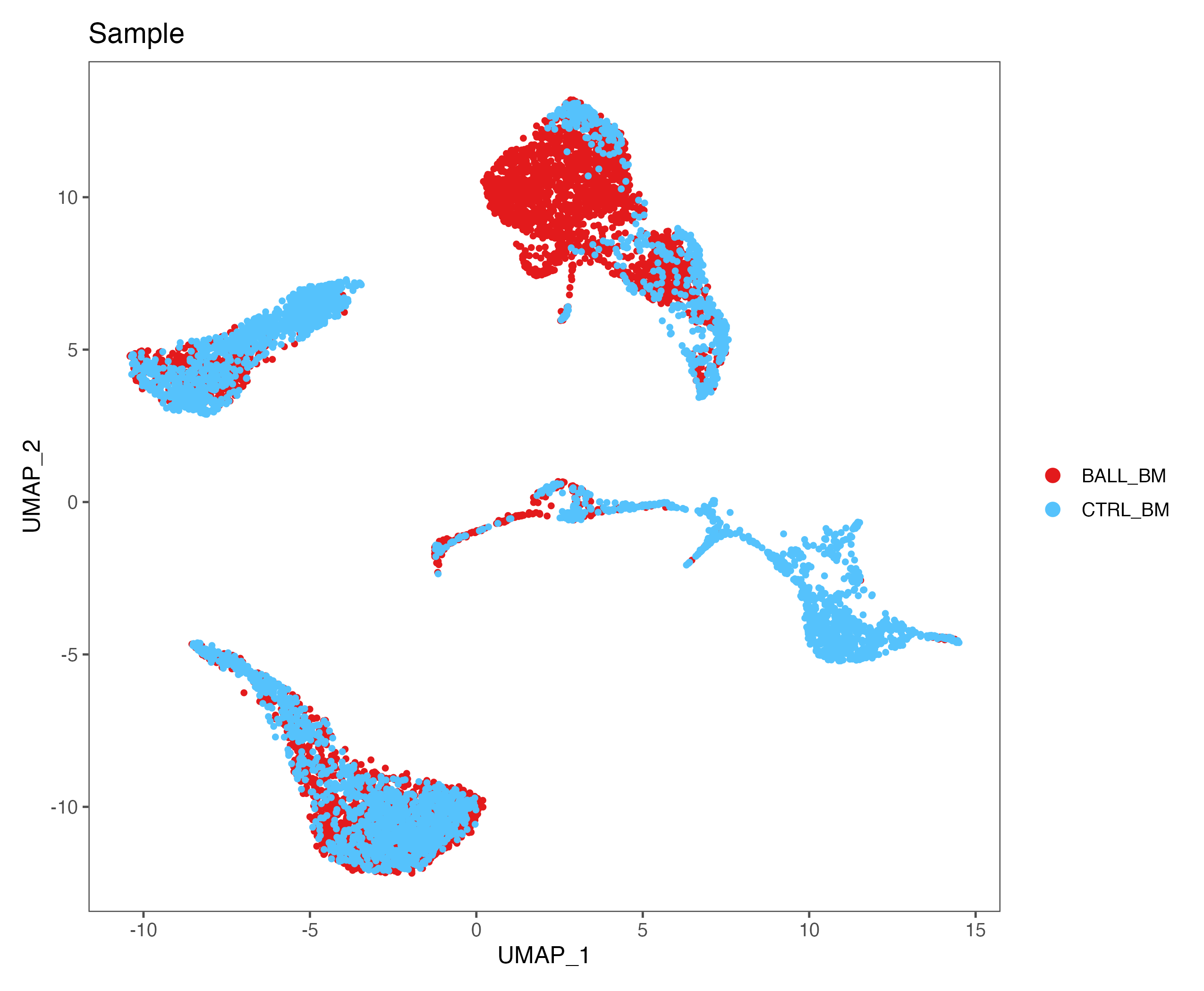
sce <- RunUMAP(sce, reduction = "harmony", dims = 1:20)
# plot
# umap
p <- DimPlot(sce, reduction = "umap", pt.size = 1,
cols = color.lib) + theme_few()
ggsave(paste0(out.path, "/5.UMAP.cluster.pdf"), p, width = 8.5, height = 7)
p <- DimPlot(sce, reduction = "umap", pt.size = 1, label = TRUE, label.size = 10,
cols = color.lib) + theme_few()
ggsave(paste0(out.path, "/5.UMAP.cluster.label.pdf"), p, width = 8.5, height = 7)
p <- DimPlot(sce, reduction = "umap", pt.size = 1, group.by = "Sample",
cols = color.lib) + theme_few()
ggsave(paste0(out.path, "/5.UMAP.sample.pdf"), p, width = 8.5, height = 7)
# tsne
p <- DimPlot(sce, reduction = "tsne", pt.size = 1,
             cols = color.lib) + theme_few()
ggsave(paste0(out.path, "/6.tSNE.cluster.pdf"), p, width = 8.5, height = 7)

p <- DimPlot(sce, reduction = "tsne", pt.size = 1, label = TRUE, label.size = 10,
             cols = color.lib) + theme_few()
ggsave(paste0(out.path, "/6.tSNE.cluster.label.pdf"), p, width = 8.5, height = 7)

p <- DimPlot(sce, reduction = "tsne", pt.size = 1, group.by = "Sample",
             cols = color.lib) + theme_few()
ggsave(paste0(out.path, "/6.tSNE.sample.pdf"), p, width = 8.5, height = 7)
#----------------------------------------------------------------------------------
#  Step11: Cell cycle
#----------------------------------------------------------------------------------
cc.genes
sce <- CellCycleScoring(sce, s.features = cc.genes$s.genes, g2m.features = cc.genes$g2m.genes)
p <- DimPlot(sce, reduction = "umap", pt.size = 1, label = FALSE,
             group.by = "Phase", cols = color.lib) + theme_few()
ggsave(paste0(out.path, "/7.CC.phase.pdf"), p, width = 8.5, height = 7)

p <- VlnPlot(sce, features = "S.Score", pt.size = 0,
             group.by = "seurat_clusters", cols = color.lib) + theme_few()
ggsave(paste0(out.path, "/7.CC.score.S.Score.pdf"), p, width = 10, height = 5)

p <- VlnPlot(sce, features = "G2M.Score", pt.size = 0,
             group.by = "seurat_clusters", cols = color.lib) + theme_few()
ggsave(paste0(out.path, "/7.CC.score.G2M.Score.pdf"), p, width = 10, height = 5)
#----------------------------------------------------------------------------------
#  Step 12: Visualization previous SingleR annotation
#----------------------------------------------------------------------------------
# umap
p <- DimPlot(sce, reduction = "umap", pt.size = 1, label = TRUE, label.size = 4,
             group.by = "CellType.BlueprintEncodeData", cols = color.lib) + theme_few()
ggsave(paste0(out.path, "/8.SingleR.umap.BlueprintEncodeData.pdf"), p, width = 9, height = 7)

p <- DimPlot(sce, reduction = "umap", pt.size = 1, label = TRUE, label.size = 4,
             group.by = "CellType.HumanPrimaryCellAtlasData", cols = color.lib) + theme_few()
ggsave(paste0(out.path, "/8.SingleR.umap.HumanPrimaryCellAtlasData.pdf"), p, width = 9, height = 7)

p <- DimPlot(sce, reduction = "umap", pt.size = 1, label = TRUE, label.size = 4,
             group.by = "CellType.NovershternHematopoieticData", cols = color.lib) + theme_few()
ggsave(paste0(out.path, "/8.SingleR.umap.NovershternHematopoieticData.pdf"), p, width = 9, height = 7)
# tsne
p <- DimPlot(sce, reduction = "tsne", pt.size = 1, label = TRUE, label.size = 4,
             group.by = "CellType.BlueprintEncodeData", cols = color.lib) + theme_few()
ggsave(paste0(out.path, "/8.SingleR.tsne.BlueprintEncodeData.pdf"), p, width = 9, height = 7)

p <- DimPlot(sce, reduction = "tsne", pt.size = 1, label = TRUE, label.size = 4,
             group.by = "CellType.HumanPrimaryCellAtlasData", cols = color.lib) + theme_few()
ggsave(paste0(out.path, "/8.SingleR.tsne.HumanPrimaryCellAtlasData.pdf"), p, width = 9, height = 7)

p <- DimPlot(sce, reduction = "tsne", pt.size = 1, label = TRUE, label.size = 4,
             group.by = "CellType.NovershternHematopoieticData", cols = color.lib) + theme_few()
ggsave(paste0(out.path, "/8.SingleR.tsne.NovershternHematopoieticData.pdf"), p, width = 9, height = 7)
#----------------------------------------------------------------------------------
#  Step 13: Finding differentially expressed features (find marker)
#----------------------------------------------------------------------------------
ident.meta <- data.frame(table(sce@meta.data$seurat_clusters))
colnames(ident.meta) <- c("Cluster","CellCount")
write.xlsx(ident.meta, paste0(out.path, "/9.CellCount.xlsx"), overwrite = T)
#   Cluster CellCount
# 1       0      2201
# 2       1      1385
# 3       2      1096
# 4       3       648
# 5       4       547
# 6       5       545

# find marker
sce <- BuildClusterTree(object = sce)
# PlotClusterTree(sce)
all.markers <- FindAllMarkers(object = sce, only.pos = TRUE, logfc.threshold = 0.1, min.pct = 0.1)
all.markers <- all.markers[which(all.markers$p_val_adj < 0.05 & all.markers$avg_log2FC > 0), ]
write.xlsx(all.markers, paste0(out.path, "/10.top.markers.xlsx"), overwrite = T)
# plot top 10 markers
all.markers <- read.xlsx(paste0(out.path, "/10.top.markers.xlsx"))
all.markers <- all.markers[which(all.markers$pct.1 > 0.25), ]
top10 <- all.markers %>% group_by(cluster) %>% top_n(n = 5, wt = avg_log2FC)
gene.list <- unique(top10$gene)
p <- DotPlot(sce, features = gene.list, dot.scale = 8, cols = c("#DDDDDD", "#003366" ), col.min = -2) + RotatedAxis()
p <- p + theme_few() + theme(axis.text.x = element_text(angle = 90, hjust = 1, vjust = 0.5, size = 14))
p <- p + theme(axis.text.y = element_text(size = 20))
p <- p + scale_size(range = c(1, 7))
p <- p + gradient_color(c("#EEEEEE","#ffb459","#e8613c","#b70909"))
ggsave(paste0(out.path, "/10.top.markers.pdf"), p, width = 20, height = 7)
#----------------------------------------------------------------------------------
# Step 14: check wellknown markers
#----------------------------------------------------------------------------------
# Expression for each cluster
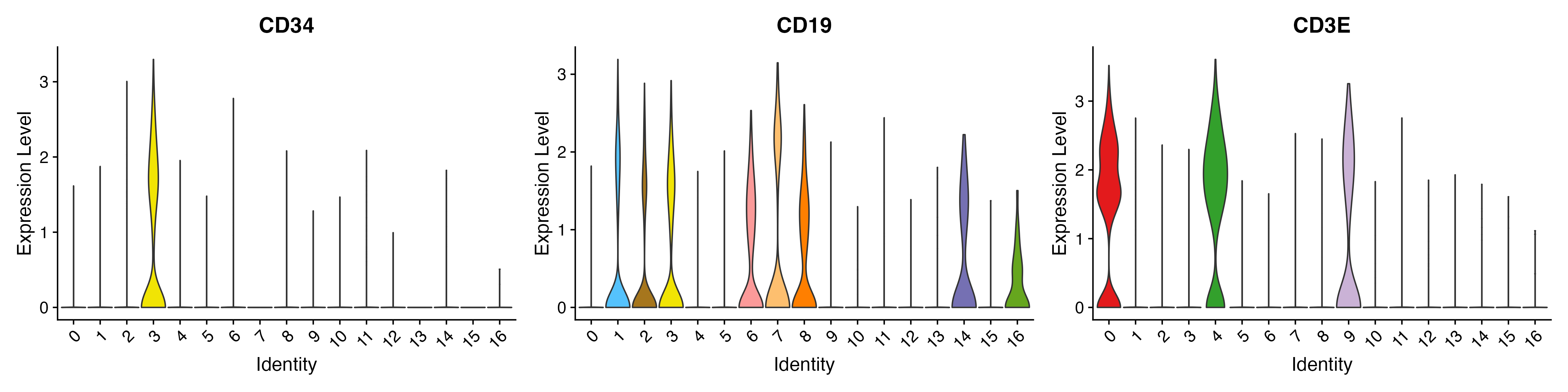
p <- FeaturePlot(object = sce, features = c("CD34","CD19","CD3E"),
cols = c("#CCCCCC", "red"), pt.size = 0.5, ncol = 3,
reduction = "umap")
ggsave(paste0(out.path, "/11.featurePlot.pdf"), p, width = 14, height = 4)

p <- VlnPlot(object = sce, features = c("CD34","CD19","CD3E"), pt.size = 0,
             cols = color.lib, slot = "data", ncol = 3)
ggsave(paste0(out.path, "/11.VlnPlot.pdf"), p, width = 16, height = 4)
## Percentage summary
ident.meta <- data.frame(sce@meta.data)
ident.info.meta <- table(ident.meta[, c("seurat_clusters", "Sample")])
ident.info.per <- ident.info.meta
# seurat_clusters BALL_BM CTRL_BM
# 0 1327 874
# 1 1381 4
# 2 466 630
# 3 350 298
# 4 13 534
plot.data <- NULL
for (i in 1:ncol(ident.info.meta)) {
plot.data.sub <- as.data.frame(ident.info.meta[, i])
colnames(plot.data.sub)[1] = "CellCount"
plot.data.sub$Percentage <- plot.data.sub$CellCount / sum(plot.data.sub$CellCount) * 100
plot.data.sub$CellType <- rownames(plot.data.sub)
plot.data.sub$Sample <- colnames(ident.info.meta)[i]
plot.data <- rbind(plot.data, plot.data.sub)
ident.info.per[, i] <- ident.info.per[, i]/sum(ident.info.per[, i])*100
}
# seurat_clusters BALL_BM CTRL_BM
# 0 27.47412008 20.85918854
# 1 28.59213251 0.09546539
# 2 9.64803313 15.03579952
# 3 7.24637681 7.11217184
# 4 0.26915114 12.74463007
# 5 7.39130435 4.48687351
write.xlsx(list(Count = ident.info.meta, Percent = ident.info.per), paste0(out.path, "/12.cluster.percentage.xlsx"), rowNames = T, overwrite = T)
## plot
order = colnames(ident.info.meta)
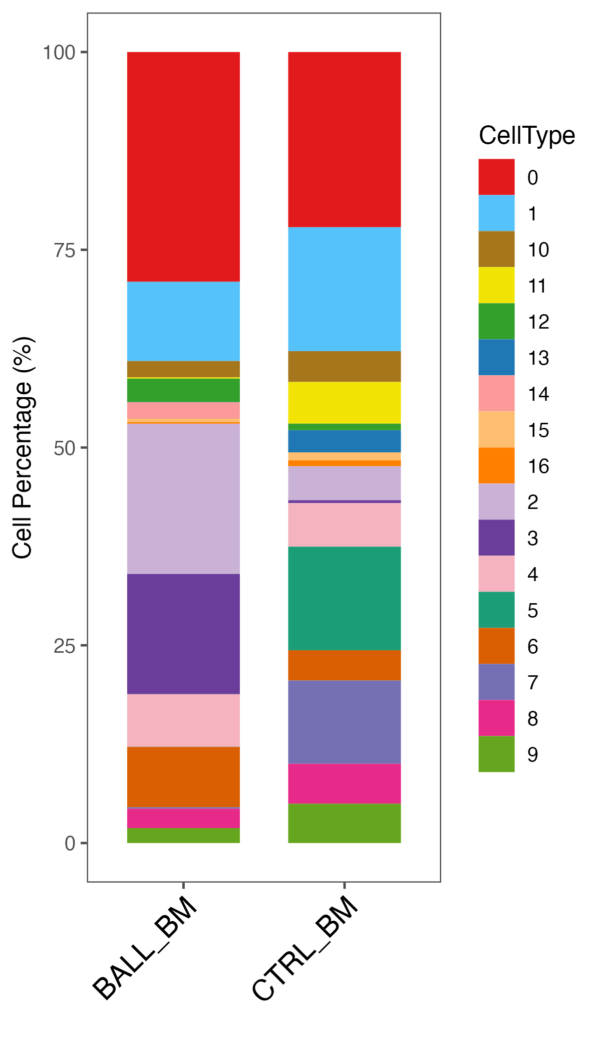
p <- ggbarplot(plot.data, x = "Sample", y = "Percentage",
fill = "CellType", color = "CellType", width = 0.7,
palette = color.lib, size = 0,
legend = "right", xlab = "", ylab = "Cell Percentage (%)",
order = order )
p <- p + theme_few()
p <- p + theme(axis.text.x = element_text(angle = 45, hjust = 1, vjust = 1, size = 14, color = "black"))
ggsave(paste0(out.path, "/12.cluster.Percentage.pdf"), p, width = 4, height = 7)
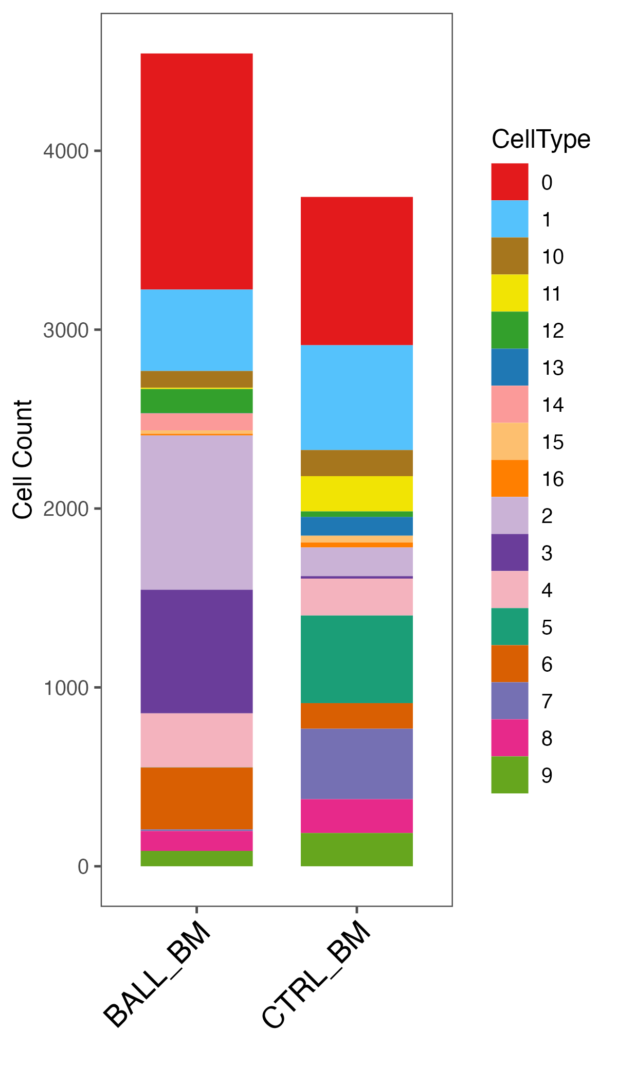
p <- ggbarplot(plot.data, x = "Sample", y = "CellCount",
          fill = "CellType", color = "CellType", width = 0.7,
          palette = color.lib, size = 0,
          legend = "right", xlab = "", ylab = "Cell Count",
          order = order )
p <- p + theme_few()
p <- p + theme(axis.text.x = element_text(angle = 45, hjust = 1, vjust = 1, size = 14, color = "black"))
ggsave(paste0(out.path, "/12.cluster.Count.pdf"), p, width = 4, height = 7)
## save object
dir.create("./output/obj",recursive = T)
saveRDS(sce, paste0("./output/obj/20231011.", "merge_BALL_CTRL", ".rds"))